JZ-TREE

← All codes

Code overview

jz-tree is a library for efficient dual tree walks with JAX and CUDA. The code includes implementations of nearest-neighbour search and friends-of-friends group finding and can easily serve as a basis for other algorithms as well.

Building on the same tree structure, jz-fmm implements the Fast Multipole Method for gravity calculations and other spatial convolutions, including differentiable N-body simulations.

Performance

The benchmark below compares a 30-nearest-neighbour search in three dimensions on a single NVIDIA A100 GPU:

Installation

The code is open source and can be installed with:

pip install 'jztree[cuda12]'   # or 'jztree[cuda13]'

Documentation and source

• Official documentation
• Code repository
• Preprint: arXiv:2604.05885

How it works

Here I will explain the main ideas behind jz-tree using a four-nearest-neighbour search. We will start with the tree structure, then work our way from a brute-force search to a dual tree walk. The important question for GPU performance is not just how many distances we calculate, but how much data we read to calculate them.

Compared with CPUs, GPUs typically offer a much larger increase in arithmetic throughput than in memory bandwidth. This means that we need to do more calculations per byte read to make full use of their computing power. Optimising an algorithm for the GPU therefore often means optimising its memory access pattern: reading neighbouring data together and reusing what we have already loaded.

The step-by-step examples below come from my ASHPC26 presentation. Use Previous and Next to go through the nearest-neighbour examples; you can also use the arrow keys while a button has focus.

Building the tree

First, we sort the particles in z-order, also called Morton order. Imagine following a path that visits one spatial region before moving to the next. This gives us a one-dimensional array in which spatial groups occupy contiguous ranges. Nearby points do not always sit next to each other in this ordering, but the particles belonging to a tree node do.

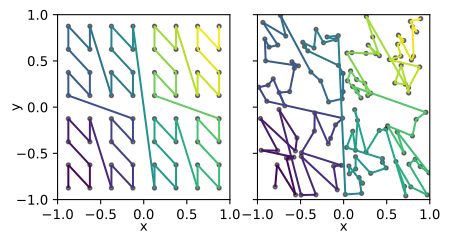Z-order gives us a spatially organised sequence, both on a regular grid (left) and for an irregular particle distribution (right). Colour follows the position in the sorted array. Figure 2 from the jz-tree paper.

We then select splitting points in the sorted array to define small leaf nodes. We respect the spatial boundaries of the z-order hierarchy and limit the number of particles per leaf. To build a coarser level, we keep a subset of those splitting points and allow more particles per node. Repeating this gives us the tree from the bottom up.

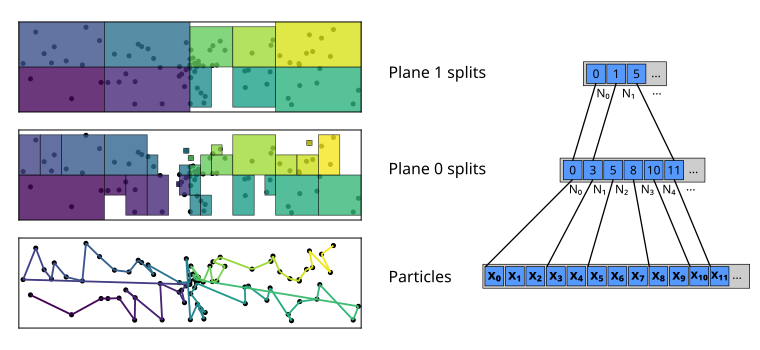The same hierarchy in space (left) and memory (right). We sort the particles in z-order, then select splitting points for the leaves and the coarser planes. Here the particle limits are four at plane 0 and twelve at plane 1. Each node’s children occupy a contiguous range. Figure 2 from the jz-fmm paper.

Why organise particles into a tree hierarchy?

• Group particles at different scales: we can work with individual particles, small groups, or larger regions as needed.
• Summarise calculations: information about a whole node can let us handle or rule out many particle interactions at once.
• Reduce the amount of work: suitable tree algorithms can achieve O(N) or O(N log N) scaling instead of checking every particle pair, depending on the problem and distribution.
• Adapt to irregular distributions: dense regions contain smaller nodes, while sparse regions can use larger ones.

What is special about our plane-based hierarchy?

• Each plane covers all particles: a tree plane is a level of the hierarchy, not a geometric cutting plane. Every particle belongs to exactly one node on each plane.
• The tree has fixed depth everywhere: every particle passes through the same number of levels, so we can organise the work as a regular sequence of plane-by-plane operations.
• Nodes can have different numbers of children: we retain the flexibility to adapt to the particle distribution within that fixed-depth structure.
• Children occupy contiguous ranges in memory: threads can read a node’s particles or children collaboratively, and we can process many nodes on the same plane in parallel.

Brute-force neighbour search

For each query point, we want the four closest source points. The query and source sets can be different. For now, the tree is only a way to organise our data; let us first consider how we would solve the problem without using it to skip any work.

The simplest approach gives each query its own thread. We go through all source points, calculate their distances, and keep the four closest candidates seen so far. Once we have four candidates, the distance to the most distant one gives us our current search radius. A closer candidate replaces that neighbour and may shrink the radius.

1 / 5 — We want the four nearest source points to the red query point. Initially, we have checked none.

2 / 5 — Read the first source position and calculate its distance to the query point.

3 / 5 — After four candidates, we have a first set of neighbours. The circle reaches the most distant of these four.

4 / 5 — Continue through the source array, replacing the most distant candidate whenever we find a closer one.

5 / 5 — After checking all 150 source points, the four remaining candidates are the four nearest neighbours.

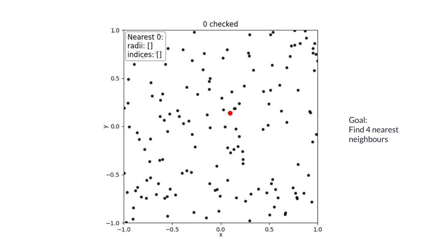
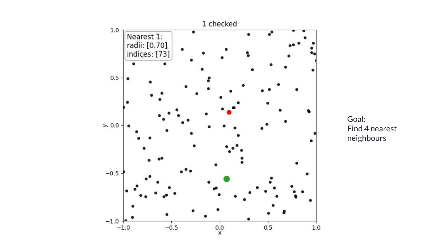
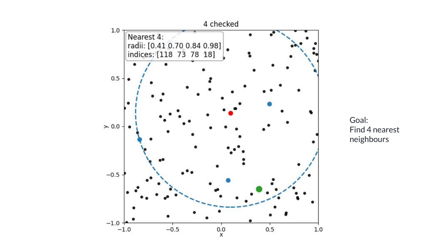
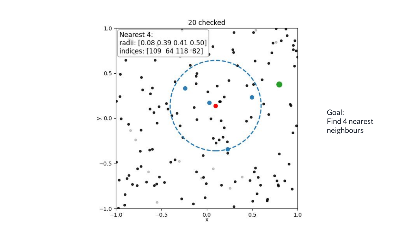
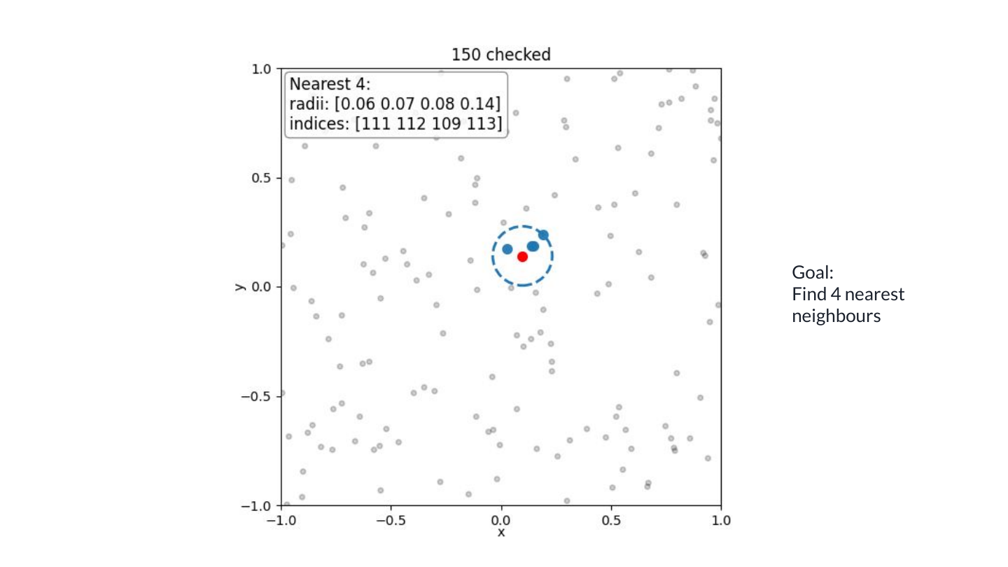
This works, but each query scans the entire source array. For N source points and Q queries, we calculate N × Q distances. If every query independently loads its sources, we also ask for the same positions over and over again.

Letting threads collaborate

Instead, give a small group of nearby queries to a thread group. Each thread still keeps its own nearest neighbours, but the threads now load a batch of source positions together. They share those positions and reuse them for all queries in the group before loading the next batch.

1 / 7 — Now find four neighbours for each red query point. Assign the nearby queries to one thread group.

2 / 7 — Each thread keeps track of the neighbours for its own query point.

3 / 7 — The threads read a batch of source positions collaboratively and share them within the group.

4 / 7 — Every query uses the same source batch. We reuse the loaded positions for several distance calculations.

5 / 7 — Move through the source groups together, updating each query's four best candidates.

6 / 7 — After visiting all source groups, each query has its own four nearest neighbours.

7 / 7 — Collaborative reads improve memory access, but we still compare every query with every source point.

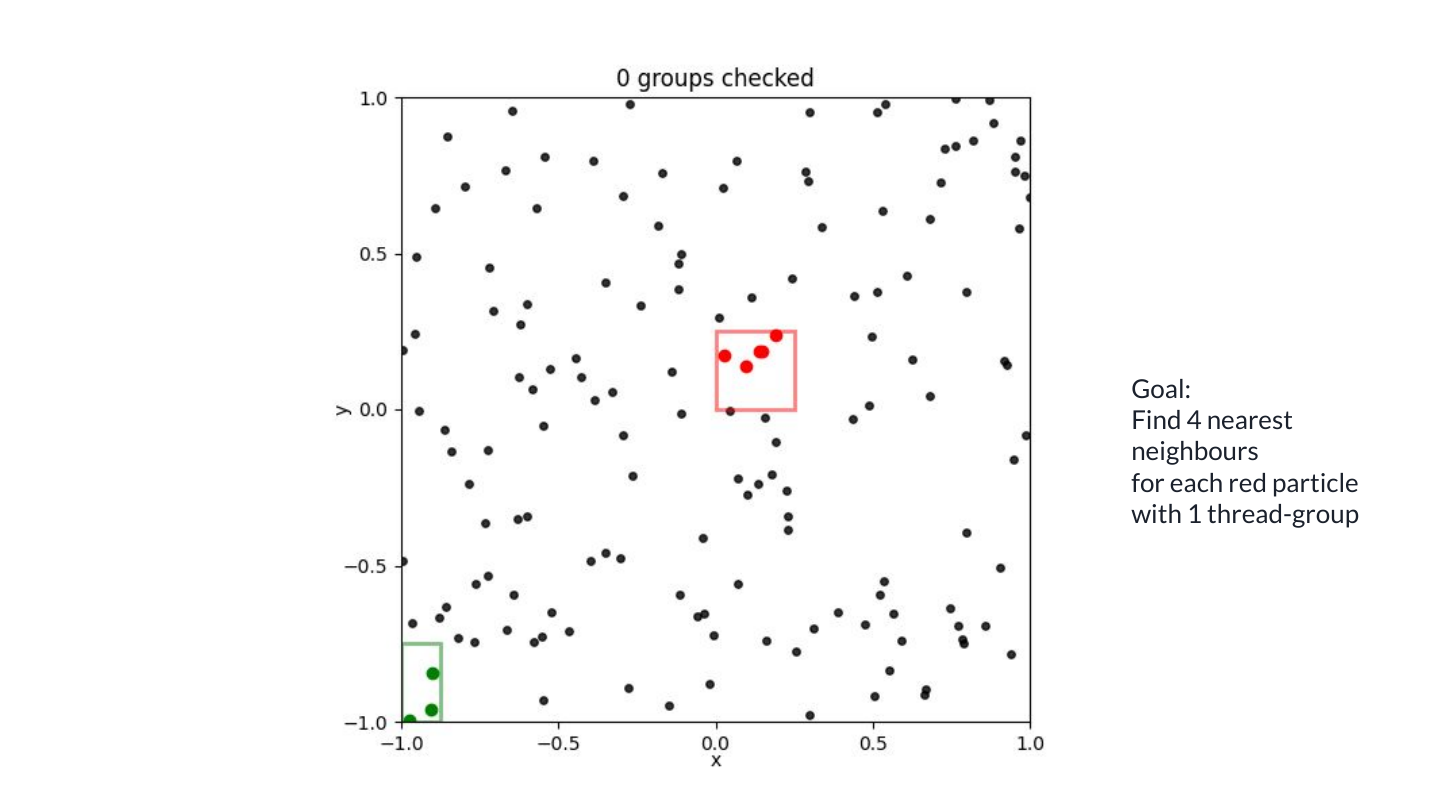
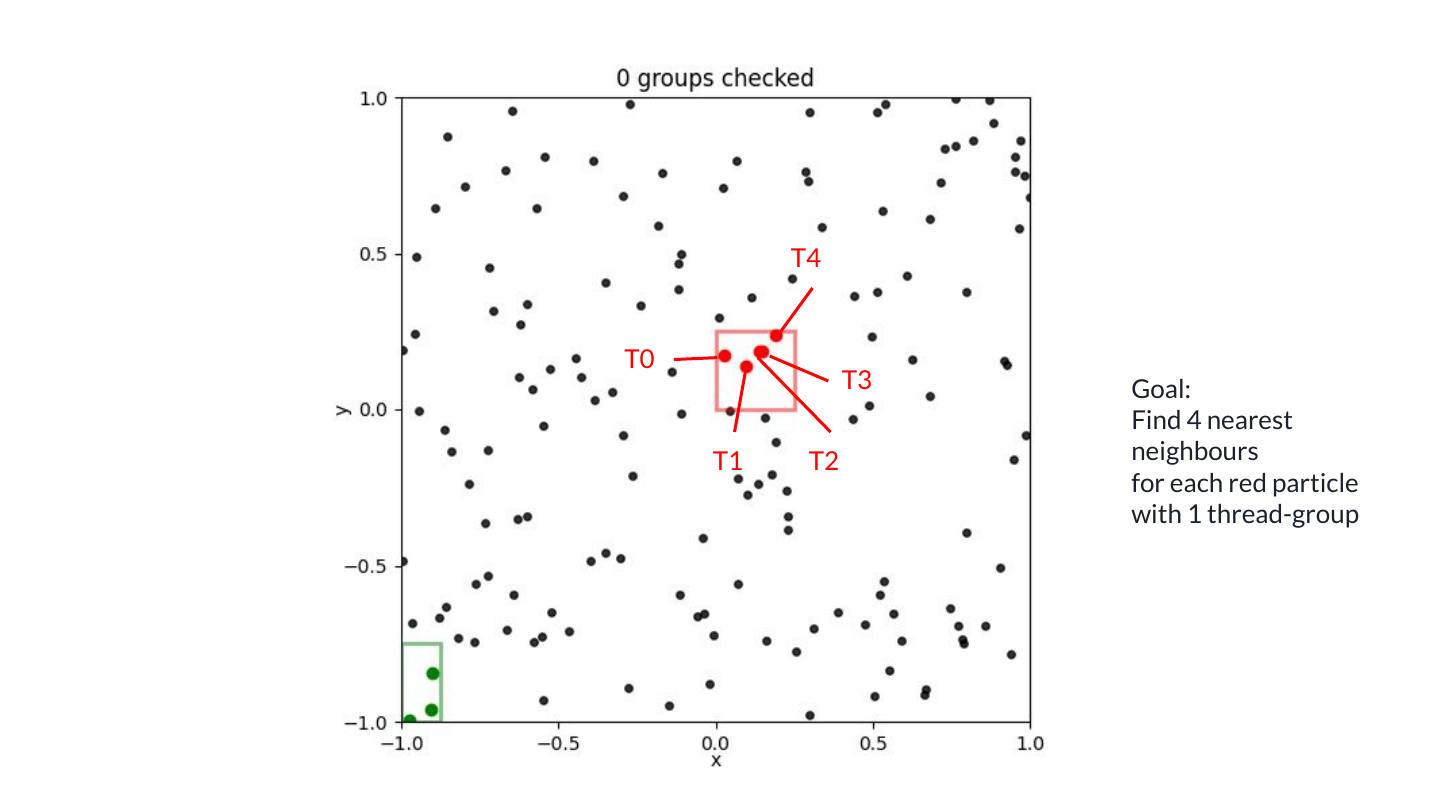
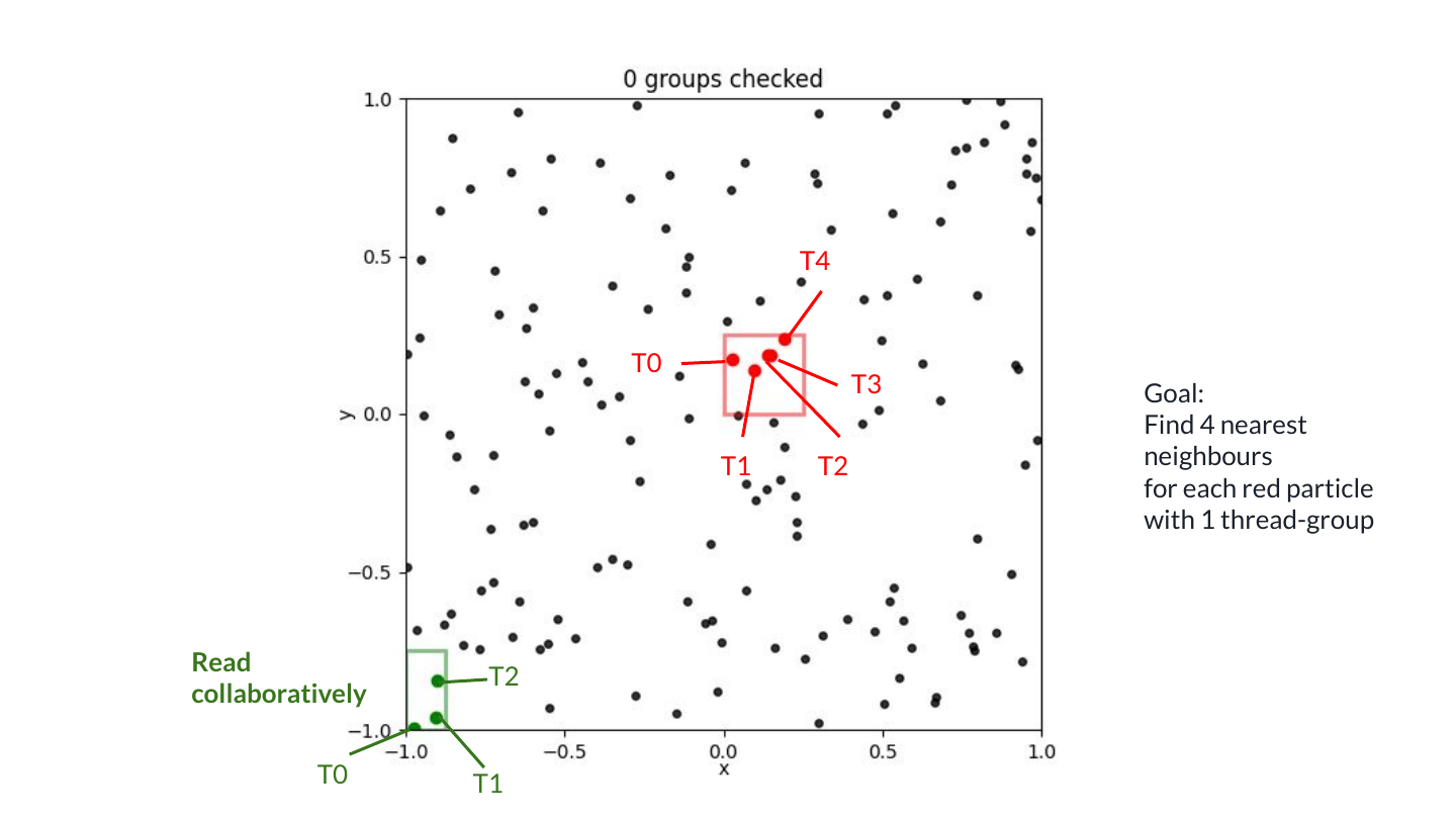
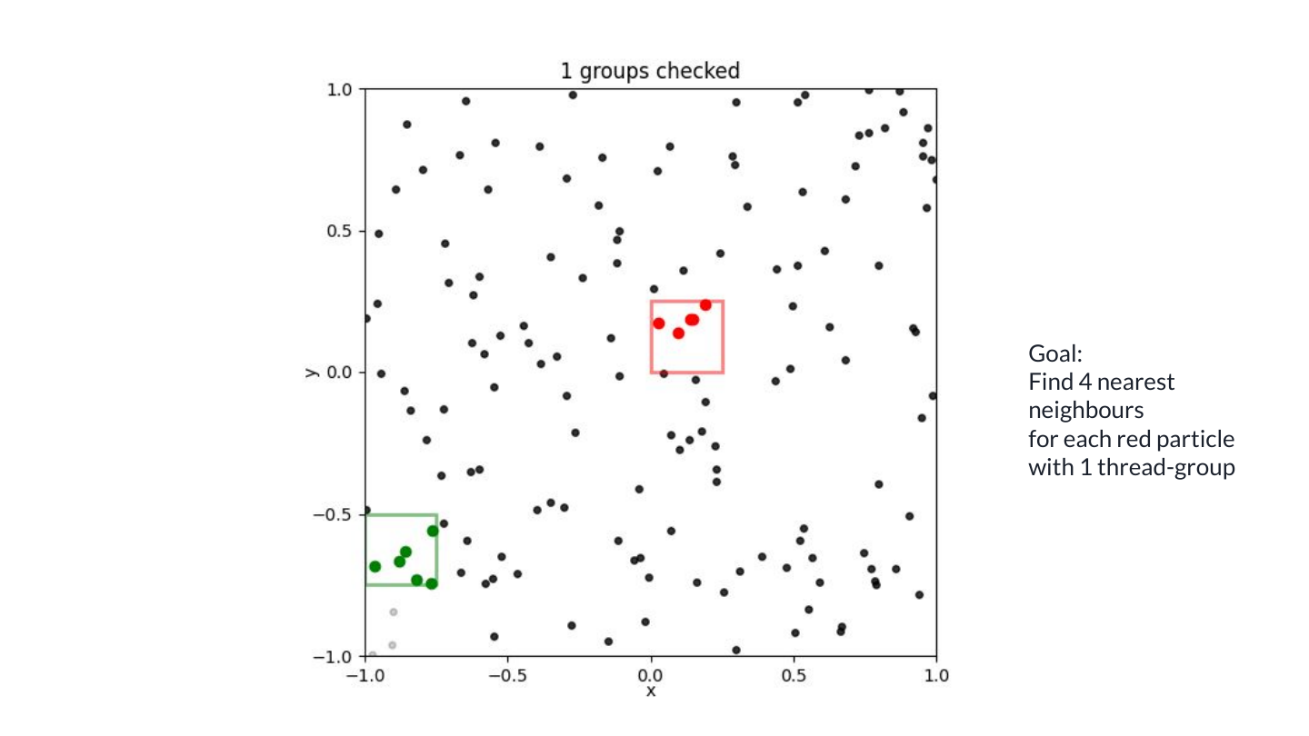
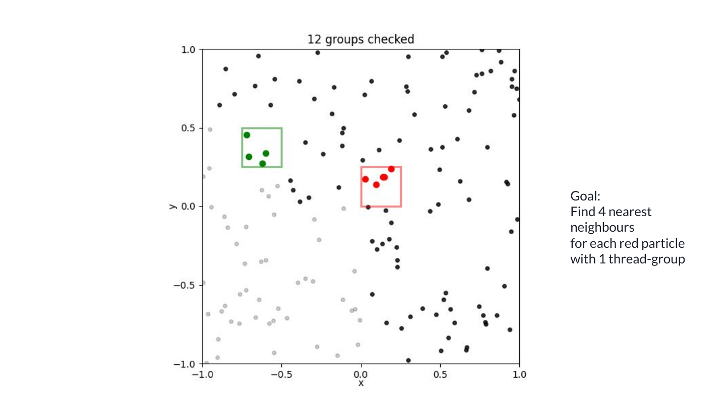
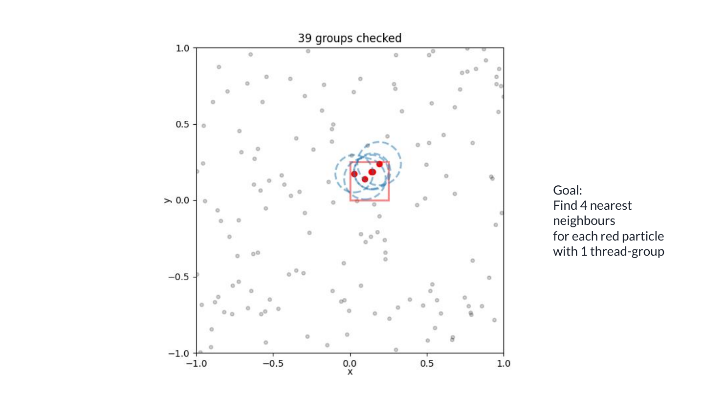
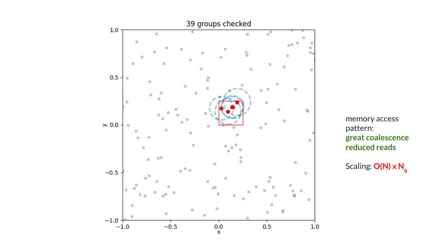
There are two benefits here. First, neighbouring threads read neighbouring addresses, which lets the GPU combine their requests into fewer memory transactions (coalesced access). Second, several queries reuse each loaded source position. With four queries, for example, one batch of source positions serves four sets of distance calculations. The exact traffic reduction depends on caching and the implementation, but the goal is to do more work with each read from global GPU memory.

For a concrete CUDA example of data reuse, NVIDIA’s guide shows how threads share a tile of data in matrix multiplication. The operation differs, but the principle is the same: load a batch once and use it for several calculations.

We still calculate N × Q distances. We have improved the memory access pattern; next, we want to avoid checking irrelevant sources altogether.

Visiting only relevant leaves

Imagine that someone gives us a list of all source leaves that might contain a nearest neighbour for any query in our red leaf. We call this an interaction list. It can include extra candidates, but it must not omit a leaf containing a required neighbour.

We can use exactly the same collaborative calculation as before, visiting only the leaves on the list. Each thread still calculates exact particle distances and keeps its own four nearest neighbours.

1 / 2 — Group the sources into tree leaves. The red leaf contains the queries that our thread group handles together.

2 / 2 — Suppose we already know which source leaves might contain a neighbour. Visit only these green leaves, sharing their particle data as before.

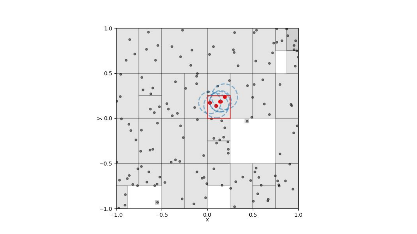
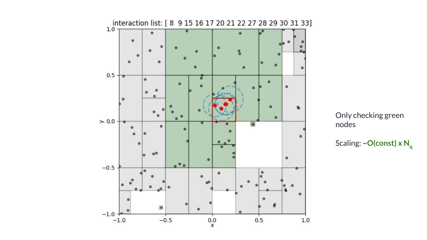
Grouping nearby queries helps twice: they share source reads, and they tend to need similar source regions. Their common interaction list can therefore stay relatively short. Its length depends on the particle distribution and the query; we should not assume that it is always constant.

Constructing interaction lists

How do we find that list without checking every particle first? We compare pairs of nodes. Let A contain our queries and B contain some source points. From the nodes’ spatial bounds, we can obtain two useful distances:

• An upper bound: every point in B lies within this distance of every location in A. If B contains at least four sources, this already gives us a radius that guarantees at least four candidates for every location in the node. We can also accumulate counts from several distinct source nodes.
• A lower bound: no point in B can lie closer than this distance to any query in A. If this exceeds our guaranteed search radius, B cannot improve any query’s four nearest neighbours, so we can discard the whole node.

1 / 8 — For the red query node, we need a list of source nodes that could contribute to any query's four nearest neighbours.

2 / 8 — An upper distance bound tells us a radius within which every query in A is guaranteed to find all n points of B.

3 / 8 — Using source counts and upper bounds, find a conservative search radius that guarantees at least four candidates for every location in the node.

4 / 8 — A lower distance bound tells us how close any pair of points in A and B could possibly be.

5 / 8 — Reject nodes whose lower bound exceeds the search radius. Keep the remaining green nodes in the interaction list.

6 / 8 — We can also assign neighbouring query nodes to a thread group when constructing these lists.

7 / 8 — Read source-node information collaboratively, then reuse it for the different query nodes.

8 / 8 — Each query node obtains its own bound and interaction list, while the threads share the source reads.

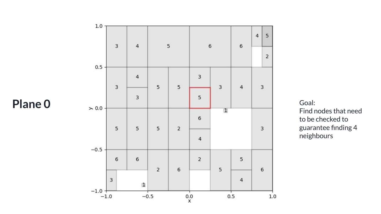
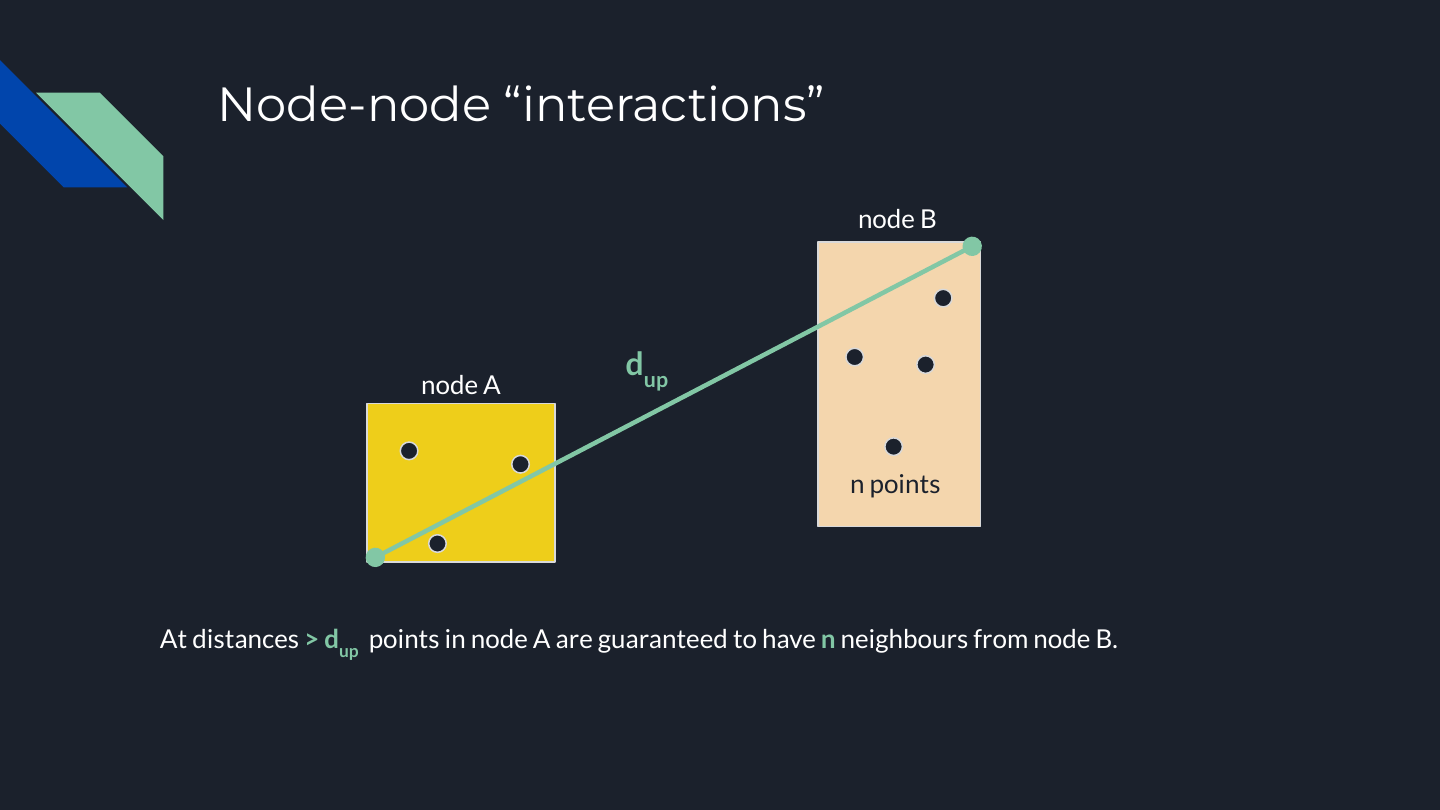
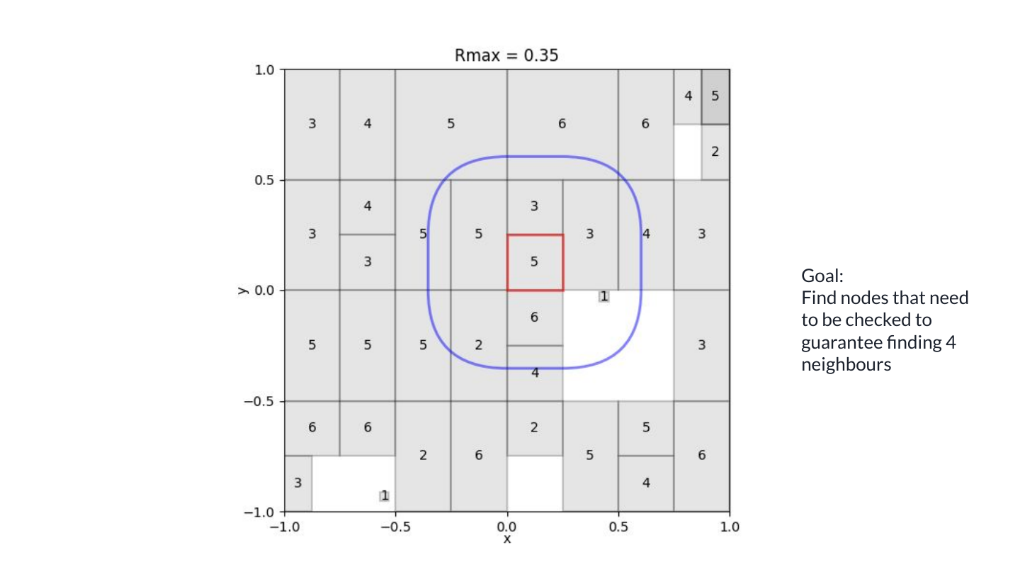
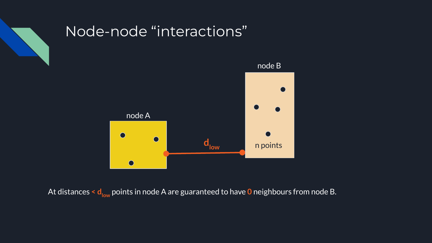
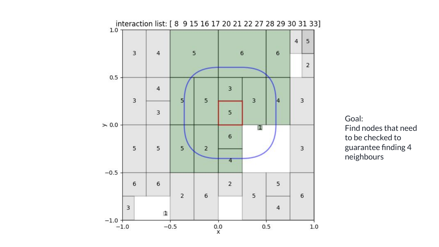
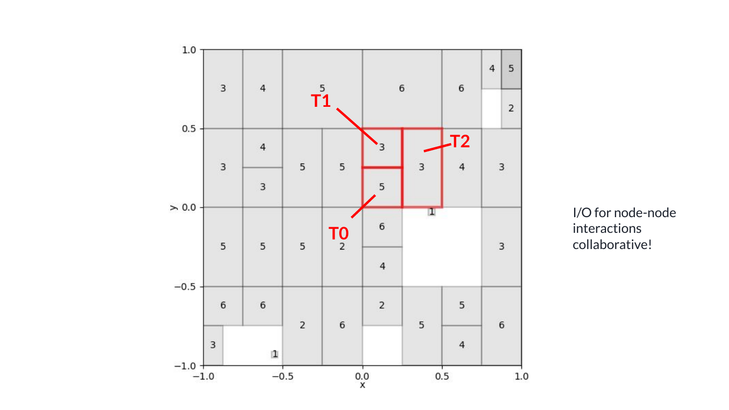
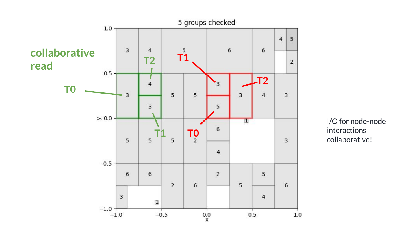
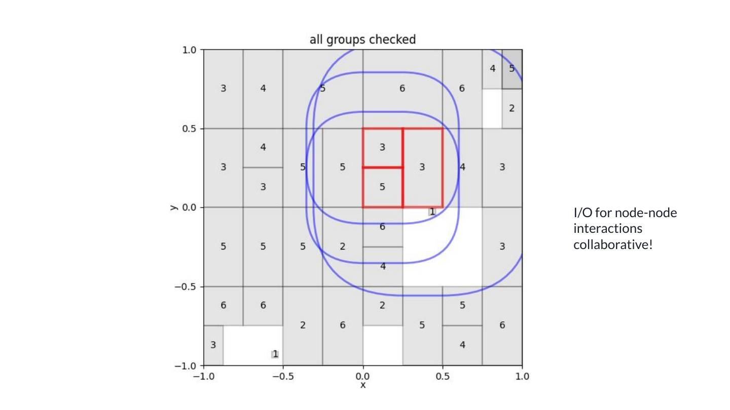
This decision is the opening criterion: do we need to examine this node pair more closely? For kNN, the criterion must conservatively retain every node that could contribute a nearest neighbour. Loose bounds mean extra work; bounds that discard a needed neighbour give a wrong result. We use node bounds to select candidates, then particle distances to determine the final neighbours.

Notice that constructing the lists is itself a collaborative calculation. Threads can load source-node bounds and counts together, then reuse them for several query nodes.

Walking down the hierarchy

We now know how to filter candidate source nodes for a query node. But checking every leaf against every other leaf would still require a lot of work. The hierarchy gives us a way out: first build interaction lists on a coarser plane.

Start at the coarsest plane, where there are few enough nodes to consider all node pairs. Apply the opening criterion and retain the relevant pairs. Then descend one plane. A child query node only needs to consider children of the source nodes retained for its parent. Refine those candidates with the opening criterion and repeat until we reach the leaves.

1 / 4 — Move up to plane 1. Each node now contains several leaves, so we can rule out larger groups at once.

2 / 4 — Construct an interaction list on this coarser plane using the same bounds and source counts.

3 / 4 — Descend to the leaves. Only children of retained coarse source nodes can contribute; test those children to refine the list.

4 / 4 — Finally, use the leaf interaction list to calculate particle distances and obtain each query's four nearest neighbours.

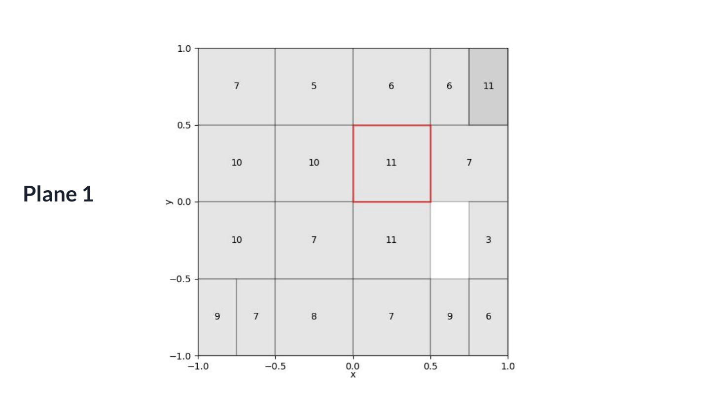
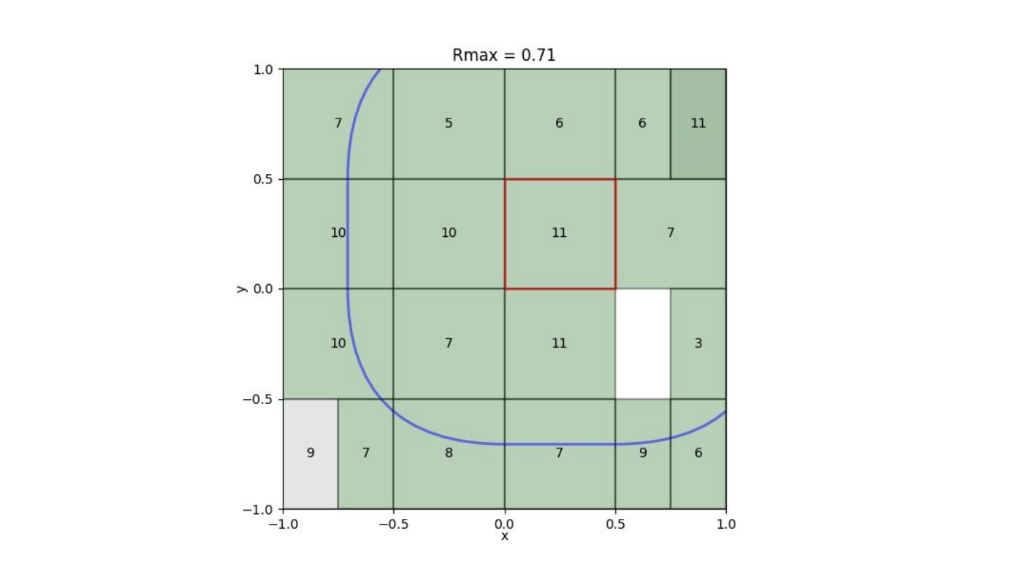
This is a dual tree walk: we traverse the query and source hierarchies together, making decisions for groups on both sides. A rejected coarse pair removes many finer comparisons at once. At the leaves, the resulting interaction lists tell our thread groups which particle batches to load.

In jz-tree, we organise this walk plane by plane. The fixed-depth hierarchy gives us a regular sequence of stages, and the contiguous child ranges let threads collaborate as we descend. The tree saves comparisons, while the data layout and shared reads make the remaining comparisons efficient on the GPU.

Defining your own dual tree walk

If you want to formulate your own algorithm as a dual tree walk, these are the most important questions:

• Node-node interactions: What part of the calculation can I do at a node-node level?
• Opening criterion: How do I decide whether I need to handle an interaction at a finer level?
• Parent-to-child relation: How do I transfer information between parent nodes and children?

Here is how we answer these questions for nearest-neighbour search, friends-of-friends, and the Fast Multipole Method:

kNN

Node-node interactions
Use distance bounds and source counts to bound the search radius for every location in a query node. Discard source nodes that cannot contribute a neighbour.

Opening criterion
Refine pairs whose minimum possible distance is within the search radius. At the leaves, calculate exact particle distances.

Parent-to-child relation
Children can use the pruning radius of their parents as a worst-case estimate.

FoF

Node-node interactions
Compare node distances with the linking length. Link whole groups when every cross-node particle pair lies within that length; discard pairs that are too far apart or already belong to the same group.

Opening criterion
Refine pairs that might contain a link but that we cannot yet link or discard as a whole.

Parent-to-child relation
Pass established group connections down to the children, together with the unresolved interactions.

FMM

Node-node interactions
Approximate the interaction through a two-sided expansion of the gravitational potential: a source multipole expansion and a local Taylor expansion in the receiving node.

Opening criterion
The approximation becomes less accurate when nodes are too close relative to their sizes. A geometric opening criterion decides whether to evaluate the interaction at a finer level.

Parent-to-child relation
Translate the local Taylor expansion of the potential from the parent's centre to each child's centre. The children then inherit the potential contributions already calculated at coarser levels.

All three algorithms pass unresolved interactions to the next finer plane. FoF additionally carries group connections, while FMM carries the field contributions already calculated on coarser planes. For FMM, an earlier upward pass also combines the children’s source multipoles into those of their parents.

For the details, see the paper sections on kNN, FoF, and FMM.