JZ-FMM
GPU-native differentiable N-body simulations with the Fast Multipole Method
Code overview
jz-fmm is a library for fast gravity calculations and differentiable N-body simulations with JAX and CUDA. It implements the Fast Multipole Method on one or multiple GPUs, building on jz-tree.
The video shows the reversibility of the simulation: we evolve the system forwards, then backwards to recover its initial state. Below, I will explain how FMM works and why reversibility helps us calculate gradients through a simulation.
Watch on YouTube · Vienna cosmology group
Documentation and source
- Official documentation
- Code repository
- Paper: jz-fmm: GPU-native differentiable N-body simulations with the Fast Multipole Method, Jens Stücker and Oskar Foldal (2026)
Why do we need the fast multipole method?
N-body simulations model the evolution of particles (e.g. stars or dark matter) through gravity. The most expensive part of such simulations is usually the calculation of forces—and there are many approaches to calculate these efficiently, all with their individual advantages and drawbacks. The fast multipole method is one of the most successful approaches in large N-body simulation codes, because it resolves forces on very small scales efficiently and scales well to very large distributed systems.
How the Fast Multipole Method works
From particle pairs to node pairs
For a direct gravity calculation, we add the contribution of every source particle to every receiving particle. This is straightforward, but doubling the particle count roughly quadruples the work.
\[\Phi(\mathbf{x}_i) = -G \sum_{j\ne i} \frac{m_j}{\lVert\mathbf{x}_i-\mathbf{x}_j\rVert}.\]Here, xᵢ is the receiving particle’s position, mⱼ and xⱼ are the source masses and positions, and G is the gravitational constant. We omit the self-interaction.
For distant groups, we can share much of this calculation. If we observe a compact mass distribution from far away, its total mass determines the leading contribution to its gravitational field. More detailed information about the distribution matters increasingly as we get closer. The Fast Multipole Method (FMM) uses this idea on both sides of the interaction: it summarises the sources and describes their potential throughout a receiving region.
Describing the source and the receiving region
Let’s look at two nodes, a source B and a receiver A, each containing many particles. We use two sets of coefficients:
- Multipole moments of B describe its mass distribution around the source centre. The lowest-order moment is the total mass; higher moments capture how the mass sits around that centre.
- Local Taylor coefficients in A describe how B’s potential varies around the receiving centre. They give us the potential, its gradient, its curvature, and higher spatial derivatives.
With each particle’s offset from the node centre \(\mathbf{s}_j=\mathbf{x}_j-\mathbf{c}_B\), the first few Cartesian mass moments are
\[\begin{aligned} M &= \sum_{j\in B}m_j,\\ \mathbf{M}^{(1)} &= \sum_{j\in B}m_j\mathbf{s}_j,\\ M^{(2)}_{\alpha\beta} &= \sum_{j\in B}m_j s_{j,\alpha}s_{j,\beta}. \end{aligned}\]These are the total mass, the dipole moment, and the second mass moment. For example, \(M^{(2)}_{xy}\) is simply the sum of \(m_j s_{j,x}s_{j,y}\). Higher moments follow the same pattern with more factors of the particle offsets. We calculate these quantities once per source node and reuse them for many receiving nodes.
At a position δx away from the receiving centre, we can write the potential as
\[\Phi(\mathbf{c}_A+\delta\mathbf{x}) \approx \Phi(\mathbf{c}_A) + \nabla\Phi(\mathbf{c}_A)\cdot\delta\mathbf{x} + \frac{1}{2}\delta\mathbf{x}^{\mathsf T}\,\mathbf{H}_{\Phi}(\mathbf{c}_A)\,\delta\mathbf{x} + \ldots\]Here, H is the Hessian of the potential. Differentiating this polynomial gives the acceleration, a = −∇Φ, at any particle position inside A. The local expansion describes contributions from accepted distant sources; we will add nearby contributions separately.
Calculating a node-node interaction
We now use B’s multipole moments and the distance between the node centres to calculate B’s contribution to the local Taylor coefficients in A. This step is called a multipole-to-local translation.
Let’s call the vector between the two centres \(\mathbf{R}=\mathbf{c}_A-\mathbf{c}_B\), with \(R=\lVert\mathbf{R}\rVert\). For the Newtonian potential, the monopole and dipole contributions give
\[\Phi_B(\mathbf{c}_A) = -G\left[ \frac{M}{R} + \frac{\mathbf{M}^{(1)}\cdot\mathbf{R}}{R^3} + \ldots\right],\]and
\[\nabla\Phi_B(\mathbf{c}_A) = G\left[ \frac{M\mathbf{R}}{R^3} - \frac{\mathbf{M}^{(1)}}{R^3} + \frac{3(\mathbf{M}^{(1)}\cdot\mathbf{R})\mathbf{R}}{R^5} + \ldots\right].\]Notice that we only need the source moments and the separation vector here, not the individual source particles.
We can add contributions from many source nodes to the same local coefficients. We then evaluate the resulting polynomial at each receiving particle’s position. This is where we save work: we share the expensive source–receiver calculation across whole groups of particles. For a fixed expansion order, the work of one translation depends on the number of expansion coefficients, rather than the number of particle pairs in the two nodes.
Try the node-node interaction below. Move the nodes closer together, then increase the expansion order. The exact view sums the individual source potentials; the approximation translates source moments into a local polynomial in A. Both views show only the potential generated by B.
Drag either node, or focus it and use the arrow keys. Switch views to compare the fields; the error always measures the approximation.
Six equal source masses generate the field; the dots in A are sample receiving particles. This 2D slice uses the 3D gravitational kernel with a small Plummer softening (ε = 0.04 node widths) to keep the potential finite when nodes overlap. The expansion keeps terms through total degree p.
The opening criterion in jz-fmm compares the nodes’ combined half-extents with the distance between their centres:
\[\theta = \frac{\lVert\mathbf{l}_A+\mathbf{l}_B\rVert} {\lVert\mathbf{c}_A-\mathbf{c}_B\rVert}, \qquad \text{open the pair if }\theta\geq\theta_{\max}.\]Here, l contains the half-width of a node along each coordinate axis, and c is its centre. We accept the node-node expansion when θ < θmax; otherwise, we move the interaction to a finer level. This is a dimensionless size-to-distance ratio, not an angle in degrees.
Combining near and far interactions
A truncated expansion works best when the nodes are small compared with their separation. We control the approximation with two choices:
- Expansion order: keeping more terms captures more of how the potential varies across the node.
- Opening criterion: a geometric test tells us whether the nodes are far enough apart. If they are too close, we evaluate their children instead.
We combine these interactions in three stages:
- Build source multipoles upwards. Calculate moments for the leaves, then translate and combine the children’s moments around their parent centres.
- Evaluate node-node interactions. Accept well-separated pairs for multipole-to-local translations and refine the remaining pairs.
- Carry the potential downwards. Translate each parent’s local Taylor expansion to its children, so they inherit the distant contributions already calculated. At the leaves, evaluate the expansions at particle positions and calculate the remaining nearby interactions directly.
In the jz-tree article I explain in more detail how to keep track of the needed interactions in a dual tree walk.
Why this works well on GPUs
The tree stores neighbouring particles and child nodes next to each other in memory. Threads can therefore load source data collaboratively and reuse it for several receiving nodes. A multipole-to-local translation then performs many calculations with those coefficients, making good use of the GPU’s arithmetic throughput. Sorting, tree construction, and the force calculation all stay on the GPU.
The discussion of collaborative reads explains the memory-access side in more detail. To see how well this works, we compare runtimes at the same force accuracy:
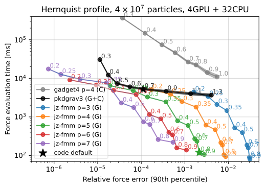 Accuracy–runtime comparison for a Hernquist sphere with 40 million particles. The measurements use one node with four NVIDIA A100 GPUs and a 32-core CPU; this is not an equal-cost CPU/GPU comparison. The curves explore expansion orders and opening angles. See Figure 9 of the paper for the setup.
Differentiating through a simulation
What do we want to differentiate?
Suppose we have a target particle distribution and want to find initial conditions that evolve into it. We define a loss that measures the mismatch between our simulation and the target. The gradient tells us how a small change in an initial position, velocity, or mass would change that loss.
We could estimate each derivative by changing one input slightly and rerunning the simulation. That quickly becomes expensive when we have many inputs. Reverse-mode differentiation instead starts with the final loss and propagates its sensitivities backwards through the calculation, obtaining gradients with respect to all those inputs in one backward pass.
Following sensitivities backwards
A simulation consists of many time steps. Each step maps the current positions and velocities to a new state. During the backward pass, we ask: how does the loss’s sensitivity to the new state translate into a sensitivity to the old one?
This is the chain rule, applied one step at a time. The operation is called a vector–Jacobian product (VJP). We do not need to construct a huge matrix of all pairwise derivatives; we only need its action on the sensitivities that arrive from the next step.
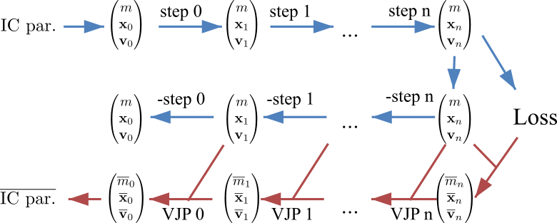 Figure 1 of the paper. The top row evolves the initial conditions forwards. The middle row reconstructs the states backwards. The bottom row carries the loss sensitivities back to the initial parameters; each VJP uses the corresponding reconstructed state.
There are two different quantities moving backwards here: the physical state and the sensitivity of the loss to that state. Reversing the particle trajectories supplies the positions and velocities needed to evaluate the derivatives. The VJP then propagates the sensitivities.
Why reversibility matters
To differentiate a time step, we need the positions and velocities we used in the forward calculation. One option is to save every state during the forward simulation. For many particles and many steps, that takes a lot of memory. With checkpointing, we save only some states and recalculate the steps in between when we need them.
In jz-fmm, we can instead reconstruct the earlier states by integrating backwards while propagating the gradients. This avoids keeping a full trajectory in memory. But we want to reconstruct the same numerical states, not merely nearby states on a plausible reverse orbit.
Ordinary floating-point operations lose information through rounding. Even a time-symmetric integration scheme does not generally recover its inputs bit for bit, and chaotic dynamics can amplify a small mismatch. We therefore use an integer-lattice integrator: positions and velocities live on an integer lattice, while the force calculation still uses floating-point arithmetic. Reversing an update subtracts the same integer increment that the forward step added.
For this to work, the force calculation must also be reproducible: revisiting the same state with the same configuration must produce the same increment. The combination allows bit-perfect reconstruction of the numerical trajectory.
Differentiating the force calculation
An important step for getting gradients is to differentiate the force calculation. In the paper, we found a surprisingly simple relation: the VJP of the fast multipole method can be evaluated very simply. One contribution comes from the next higher derivative in the original evaluation, and another contribution corresponds to a fast multipole method with the force sensitivities acting as dipole moments. So basically any implementation of the FMM can easily be used for differentiable simulations!
Example: reconstructing a satellite
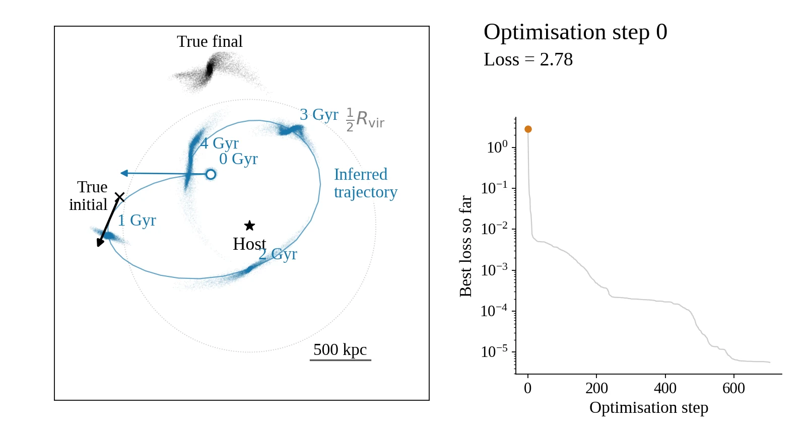
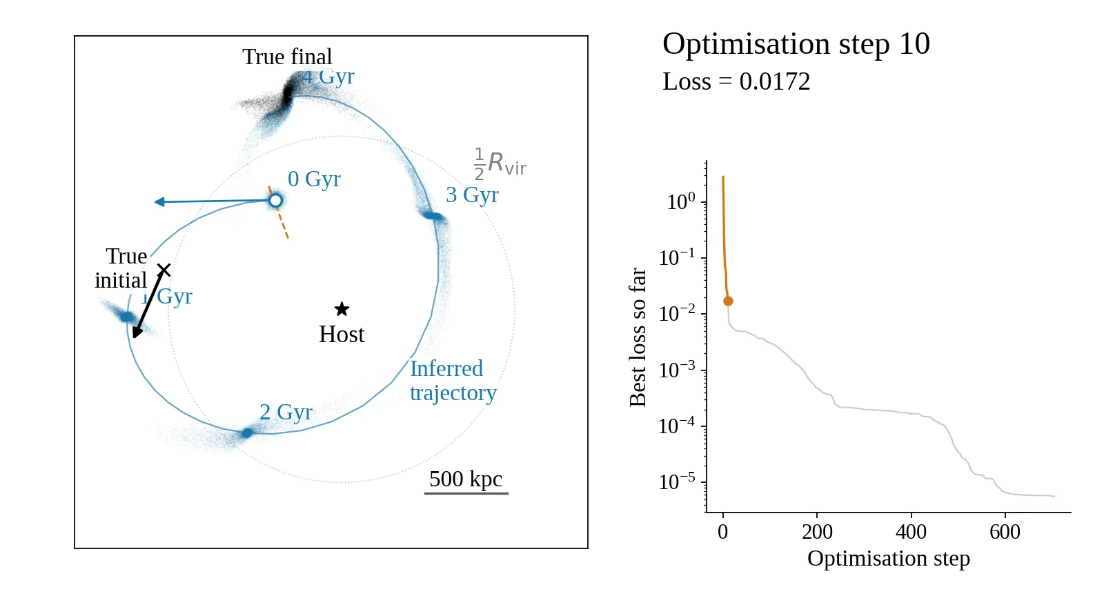
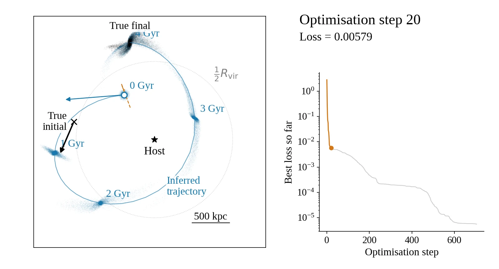
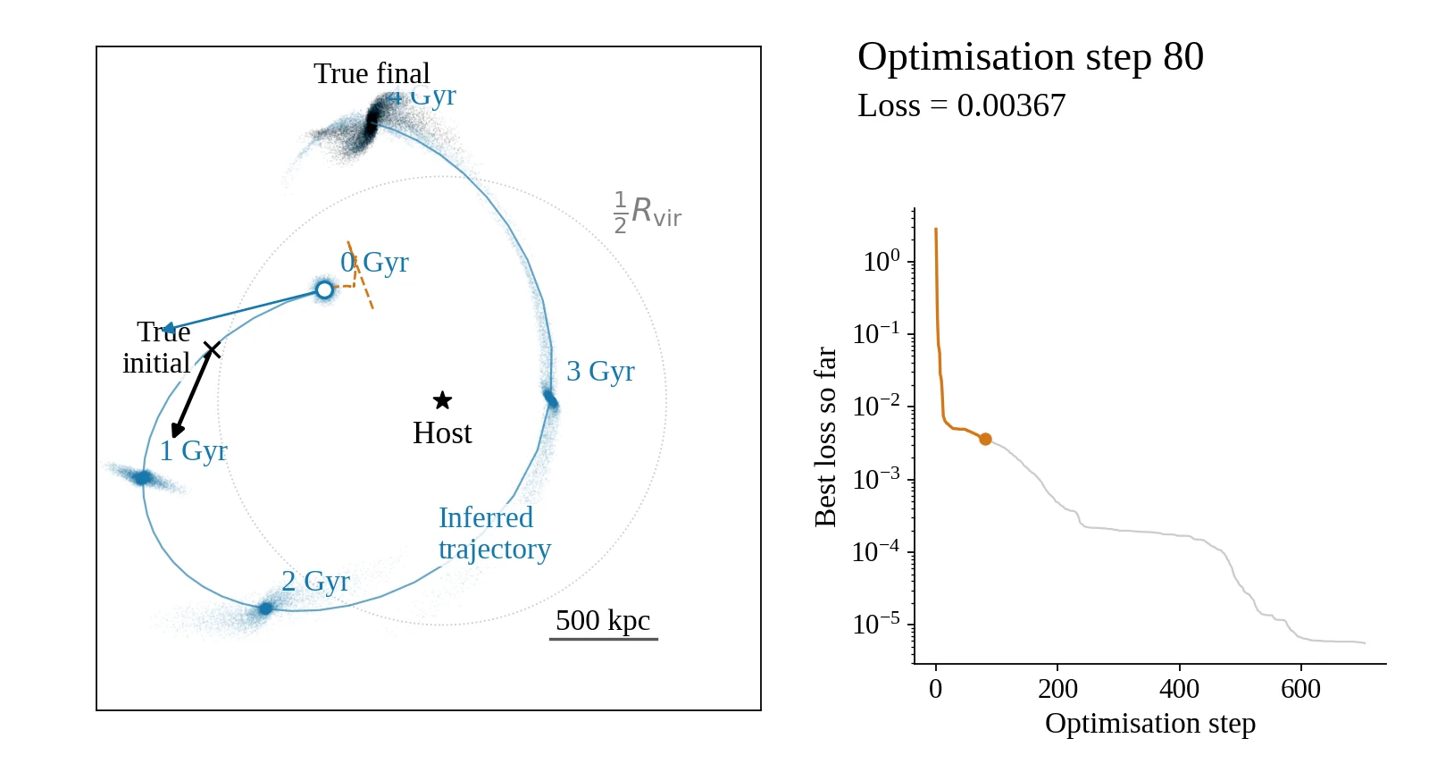
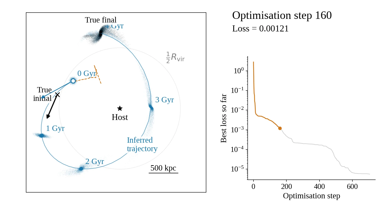
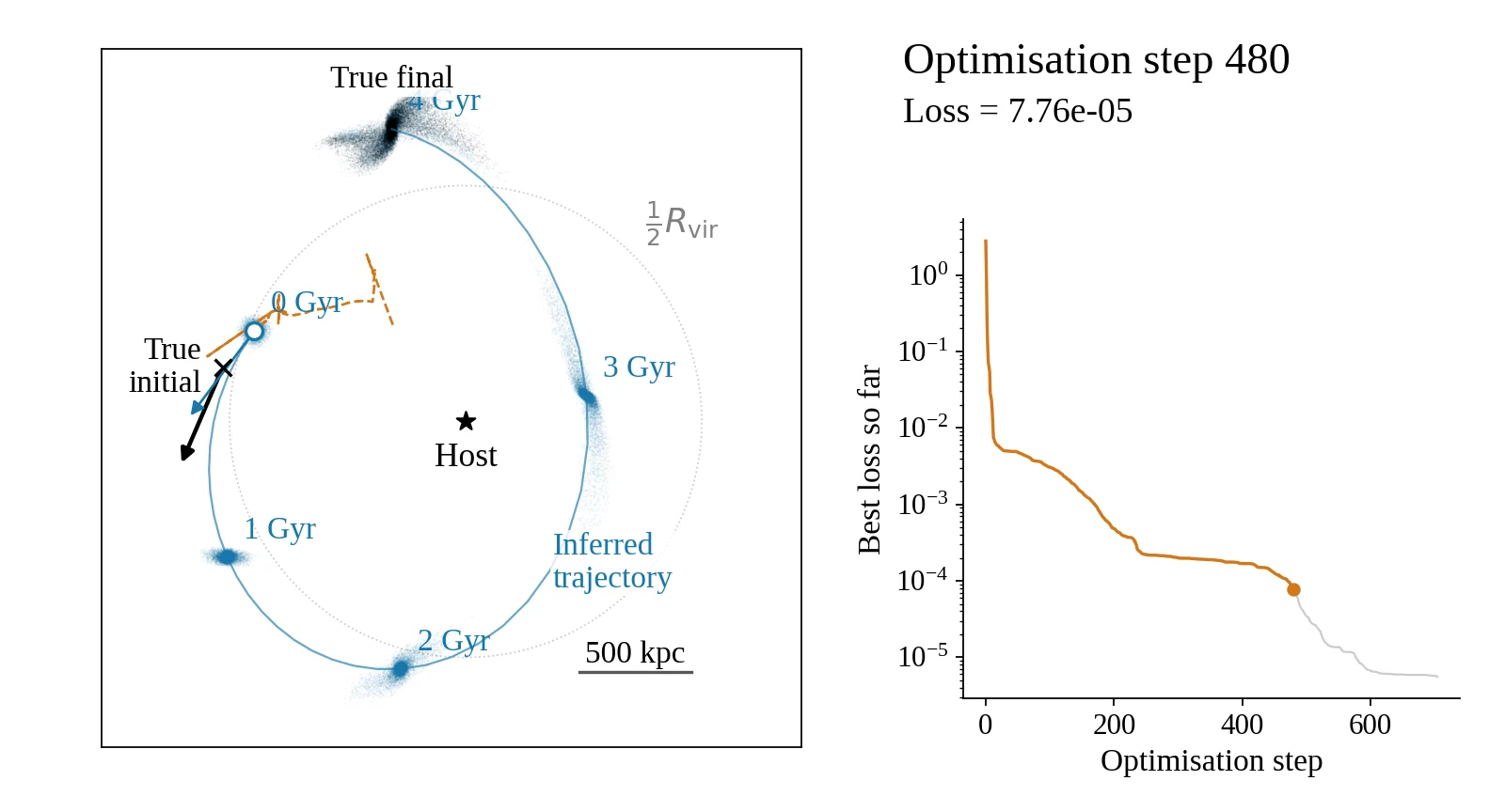
We can use these gradients to reconstruct a satellite’s orbit from its tidal debris. Starting from the final particle distribution, we assume a model for the satellite’s initial internal structure and optimise its initial centre-of-mass position and velocity.
At each iteration, we simulate the satellite, measure the mismatch with the target, and propagate the loss gradients back to the initial parameters. We update the parameters and repeat. The tidal debris constrains the earlier orbit beyond what we could learn from the final centre-of-mass position alone.
The flipchart follows seven stages of this optimisation in a known host potential. Each frame shows the full 0–4 Gyr evolution for one guess at the initial conditions, shown in the x–y projection. Black particles mark the final target; blue particles show the simulated satellite at successive times. The orange dashed line tracks the guesses for the initial position, not a physical orbit. The curve on the right shows the best loss reached so far.
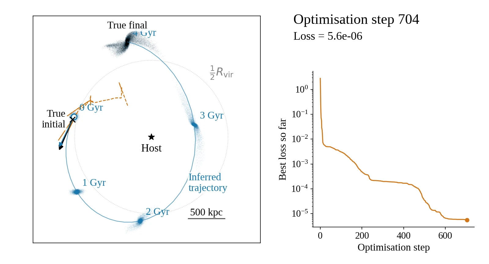
However, this kind of optimization is still somewhat tricky, because the loss landscape contains many local minima corresponding to sub-optimal solutions — so that not every gradient descent will converge to the right solution. Learning how to optimize well under such conditions will be an important topic of future research. We are only beginning to explore what differentiable simulations can tell us about the dynamical history of the Universe!