Quickstart
Nearest neighbour search
To get started, let’s create a random uniform distribution and find some neighbours!
import jax
import jax.numpy as jnp
import jztree as jz

# self-query
pos = jax.random.uniform(jax.random.key(0), shape=(int(1e7), 3))

rnn, inn = jz.knn.knn.jit(pos, k=4)

print("Self-query:", rnn.shape, inn.shape)
print(rnn[0])
print(inn[0])
Self-query: (10000000, 4) (10000000, 4)
[0.         0.00211055 0.00308441 0.0039642 ]
[      0 6307584 5332499 2674456]
or with a separate set of query positions:
posq = jax.random.uniform(jax.random.key(1), shape=(int(5e6), 3))

rnn, inn = jz.knn.knn.jit(pos, k=4, part_query=posq)
print("Separate query:", rnn.shape, inn.shape)
print(rnn[0])
print(inn[0])
Separate query: (5000000, 4) (5000000, 4)
[0.00304076 0.00344077 0.00382814 0.00440932]
[1295882 1951754 8741135 4396358]
That’s it already! The code has calculated the radii and the indices of the nearest neighbours of every particle.
As usual in jax, it is important to just-in-time (jit) compile functions to get good performance. Functions in jz-tree never use a @jax.jit decorator, to make it easier to debug them. However, for convenience we have added a .jit attribute that provides a jitted instance. E.g. if you check the jztree.knn module, just after the knn function you will find something like this:
knn.jit = jax.jit(knn, static_argnames=("k", "boxsize", "result", "reduce_func", "output_order", "cfg"))
Of course you may instead use your own jax.jit, for example:
import time

@jax.jit
def myneighbours(seed):
    pos = jax.random.uniform(jax.random.key(0), shape=(int(1e7), 3))
    return jz.knn.knn(pos, k=8)

t0 = time.perf_counter()
rnn, inn = myneighbours(seed=0)
t1 = time.perf_counter()
rnn2, inn2 = myneighbours(seed=1)
t2 = time.perf_counter()

print(f"Dt1 = {t1-t0:.2f}s, Dt2 = {t2-t1:.2f}s")
Dt1 = 2.86s, Dt2 = 0.22s
As usual in jax, the first time we run a jitted function, it will take extra-time to compile. Subsequent executions are much faster! (Timings are from my Laptop with a mobile NVIDIA 4070.)
Let’s verify by comparing to scipy’s KDTree (you may need to install it with pip install scipy)
from scipy.spatial import KDTree
import numpy as np

pos = jax.random.uniform(jax.random.key(0), shape=(int(1e7), 3))
jz.knn.knn.jit(pos, k=8) # discard compilation for profiling

t0 = time.perf_counter()
rnn, inn = jz.knn.knn.jit(pos, k=8)
t1 = time.perf_counter()
kdtree = KDTree(np.array(pos))
rnn2, inn2 = kdtree.query(pos, k=8, workers=8)
t2 = time.perf_counter()

print("All radii identical", np.allclose(rnn, rnn2))
print("Fraction of indices different:", np.mean(inn != inn2))
print("Radius collision fraction:", np.mean(rnn[:,1:] == rnn[:,:-1]))
print(f"jz-tree: {t1-t0:.2f}s, scipy: {t2-t1:.2f}s")
All radii identical True
Fraction of indices different: 2e-07
Radius collision fraction: 4.4285713e-07
jz-tree: 0.27s, scipy: 19.63s
Quite a speed-up!
Note that the results agree perfectly within the margin of error: all neighbour radii are exactly identical, but a very small number of indices differ. This is because for 10^7 particles, we already get a notable number of floating-point collisions (where two or more radii in a neighbour list are identical at machine precision). scipy and jz-tree have different tie-breaking behaviour. Feel free to verify that for each differing index, there is a second particle at the same radius.
Friends-of-friends groups
Next, let’s find some friends-of-friends clusters. For convenience, the output from a 2D cosmological N-body simulation (run with DISCO-DJ) is included in the repository. It has $128^2$ particles with a boxsize of 100.
from jztree_utils.ics import cosmo_2d_sample

pos = cosmo_2d_sample()
print(pos.shape)
mean_sep = 100./128

posz, igroup = jz.fof.fof_labels.jit(pos, rlink=0.2*mean_sep, boxsize=100.0)

print(posz.shape, igroup.shape)
print(igroup[0:40])
(16384, 2)
(16384, 2) (16384,)
[ 0  1  2  3  4  5  6  7  6  9 10 11 12 13 14 15 16 16 16 16 20 21 22 23
 24 16 16 27 27 23 30 27 27 33 34 35 35 35 38 39]
Note that jztree.fof.fof_labels outputs positions and group labels in z-order. For convience, the
single-GPU version shown here also supports restoring the input ordering (output_order="input"). However,
this is not really a feasible option in the multi-GPU scenario where it is best to continue working
with the re-ordered particles.
The igroup labels point towards the first particle that is part of the same group. Many particles just point to themselves which means that they are a single-particle group.
Let’s visualize this data:
posz, igroup = jz.fof.fof_labels.jit(pos, rlink=0.2*100./128, boxsize=100.)

count = jnp.zeros_like(igroup).at[igroup].add(1)

import matplotlib.pyplot as plt
plt.scatter(posz[:,0], posz[:,1], marker=".", alpha=0.2, color="black")

sel = count[igroup] > 10
color = plt.get_cmap("rainbow")((igroup[sel] % 133) / 133)
plt.scatter(posz[sel,0], posz[sel,1], c=color, marker=".", alpha=0.2);
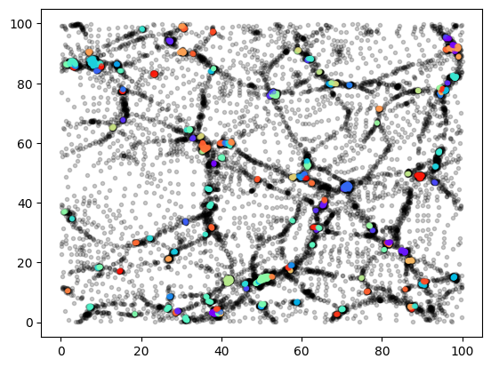
Here we have drawn only coloured particles that are in a group with more than 10 particles. The operation
count = jnp.zeros_like(igroup).at[igroup].add(1)
counts the particles in each group. We’ll see more sophisticated catalogue reductions later.
We may again wish to test our output against another library. Let’s setup a larger problem in three dimensions. (Note: By default, jz-tree supports FoF in 2 and 3 dimensions, but if you need a different dimension, you can easily add it, by recompiling from sources).
Running the following requires installing hfof – which is as far as I know the fastest publicly available single-CPU FoF library:
import hfof

pos = jax.random.uniform(jax.random.key(0), shape=(int(1e7), 3))
mean_sep = np.cbrt(1./len(pos))

jz.fof.fof_labels.jit(pos, rlink=0.7*mean_sep, boxsize=1.0) # discard jit-compilation for profiling

t0 = time.perf_counter()
posz, igroup = jz.fof.fof_labels.jit(pos, rlink=0.7*mean_sep, boxsize=1.0)
t1 = time.perf_counter()
ihfof = hfof.fof(np.array(posz), 0.7*mean_sep, boxsize=1.)
t2 = time.perf_counter()

print("jz-tree:", igroup[0:20])
print("hfof:", ihfof[0:20])
print("labels consistent:", jz.fof.fof_is_superset(igroup, ihfof), jz.fof.fof_is_superset(ihfof, igroup))
print(f"Dt1 = {t1-t0:.2f}s, Dt2 = {t2-t1:.2f}s")
Loading libhfof - C functions for FoF calculations /home/jens/.virtualenvs/uvjax/lib/python3.12/site-packages/hfof/../build/libhfof.cpython-312-x86_64-linux-gnu.so
jz-tree: [ 0  1  0  0  4  5  6  6  8  8  8 11 11  1 14 14 14 17 18 19]
hfof: [  23968     141   23968   23968       0   23846   23847   23847   23969
   23969   23969       1       1     141     142     142     142 4267019
 4267018 4267020]
labels consistent: True True
Dt1 = 0.11s, Dt2 = 4.47s
Again, a significant speed-up – though the performance of hfof is also quite impressive, given the limited hardware used!
Note that the labels differ, but they represent the same groups. This is verified by calling the jz.fof.fof_is_superset function in both directions.
Friends-of-friends catalogues
Usually FoF algorithms are run as a preparation step to create group catalogues that summarize FoF groups. This is also supported in jz-tree. To allow a convenient group-wise access to the particles they are brought into group order. To simplify visualization, we again use the cosmo 2D dataset:
pos = cosmo_2d_sample()

part = jz.data.ParticleData(
    pos = pos,
    mass = 1., # mass may be a constant or an array with number of particles
    vel = jax.random.normal(jax.random.key(0), pos.shape)
)

cfg = jz.config.FofConfig()
cfg.catalogue.npart_min = 10
mean_sep = 100./128
partf, cata = jz.fof.fof_and_catalogue.jit(part, rlink=0.2*mean_sep, boxsize=100., cfg=cfg)

print("catalogue num, shape:", cata.ngroups, cata.mass.shape)

cata = jz.data.squeeze_catalogue(cata)

print("squeezed catalogue num, shape:", cata.ngroups, cata.mass.shape)

plt.scatter(partf.pos[:,0], partf.pos[:,1], marker=".", alpha=0.2, color="black")

color = plt.get_cmap("viridis")(np.log10(cata.mass) / 2.5)
plt.scatter(cata.com_pos[:,0], cata.com_pos[:,1], c = color,
            s=200.*cata.com_inertia_radius**2, marker="o", alpha=0.8)

imax = np.argmax(cata.count)
pmax = partf.pos[cata.offset[imax]: cata.offset[imax]+cata.count[imax]]
plt.scatter(pmax[:,0], pmax[:,1], marker=".", color="red", alpha=0.1);
catalogue num, shape: 164 (1639,)
squeezed catalogue num, shape: 164 (164,)
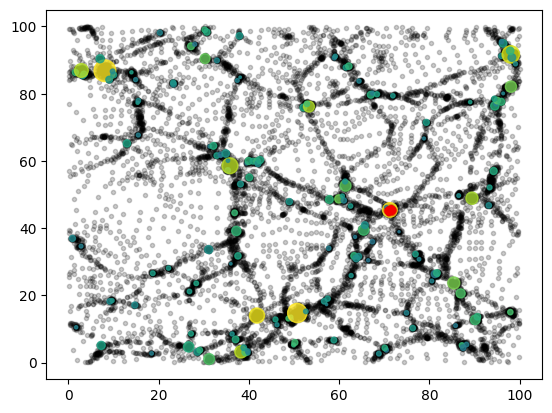
This example shows a few relevant details:
To be able to calculate group properties like masses or velocities, we should input a particle data structure with those fields.
We create and pass a config object to configure the minimal number of particles for groups (default is 20). Many functions in jz-tree have such a config interface for defining lower-level details.
jztree.fof.fof_and_catalogue()returns particles in group-prder and an instance of the dataclassjztree.data.FofCatalogue.The returned catalogue is larger than the actual number of groups. This is necessary, because the number of groups is data-dependent, but allocations need to be known at jit-compile time. jz-tree uses a worst-case estimate of the allocation size.
The function
jztree.data.squeeze_catalogue()can be used to squeeze the catalogue. (This cannot be done inside of a jitted context.)We plot the haloes centers, with size given by their inertia radius and coloured by their mass. You can find all available fields (here)
Particles can be accessed per group as a continuous range
cata.offset[gid]: cata.offset[gid]+cata.count[gid]. Here, we have plotted the particles of the most massive halo in red.
Error handling
If you are going far enough away from the scenarios that we have tested, you may sometimes encounter error messages like the following:
import jax
import jztree as jz

pos = jax.random.uniform(jax.random.key(0), shape=(50000, 3))
rnn, inn = jz.knn.knn.jit(pos, k=2000)
ERROR:2026-04-05 00:14:06,135:jax._src.callback:442: jax.io_callback failed
Traceback (most recent call last):
  File "/home/jens/.virtualenvs/uvjax/lib/python3.12/site-packages/jax/_src/callback.py", line 440, in io_callback_impl
    return tree_util.tree_map(np.asarray, callback(*args))
                                          ^^^^^^^^^^^^^^^
  File "/home/jens/.virtualenvs/uvjax/lib/python3.12/site-packages/jax/_src/callback.py", line 70, in __call__
    return tree_util.tree_leaves(self.callback_func(*args, **kwargs))
                                 ^^^^^^^^^^^^^^^^^^^^^^^^^^^^^^^^^^^
  File "/home/jens/repos/jz-tree/src/jztree/jax_ext.py", line 199, in _raise
    raise exc(txt)
RuntimeError:
======== Relevant Error Message =========
RuntimeError at /home/jens/repos/jz-tree/src/jztree/knn.py:98:
The interaction list allocation is too small. (need: 693225, have: 533760)
Hint: increase alloc_fac_ilist at least by a factor of 1.3
 Trace (last 12, tracing time, most recent call last):
-----------------------------------------
  File "/home/jens/.virtualenvs/uvjax/lib/python3.12/site-packages/jax/_src/api_util.py", line 303, in _argnums_partial
  File "/home/jens/repos/jz-tree/src/jztree/knn.py", line 273, in knn
  File "/home/jens/repos/jz-tree/src/jztree/knn.py", line 186, in _knn_dual_walk
  File "/home/jens/.virtualenvs/uvjax/lib/python3.12/site-packages/jax/_src/traceback_util.py", line 195, in reraise_with_filtered_traceback
  File "/home/jens/.virtualenvs/uvjax/lib/python3.12/site-packages/jax/_src/lax/control_flow/loops.py", line 2438, in fori_loop
  File "/home/jens/.virtualenvs/uvjax/lib/python3.12/site-packages/jax/_src/traceback_util.py", line 195, in reraise_with_filtered_traceback
  File "/home/jens/.virtualenvs/uvjax/lib/python3.12/site-packages/jax/_src/lax/control_flow/loops.py", line 251, in scan
  File "/home/jens/.virtualenvs/uvjax/lib/python3.12/site-packages/jax/_src/lax/control_flow/loops.py", line 236, in _create_jaxpr
  File "/home/jens/.virtualenvs/uvjax/lib/python3.12/site-packages/jax/_src/interpreters/partial_eval.py", line 2309, in trace_to_jaxpr
  File "/home/jens/.virtualenvs/uvjax/lib/python3.12/site-packages/jax/_src/lax/control_flow/loops.py", line 2324, in scanned_fun
  File "/home/jens/repos/jz-tree/src/jztree/knn.py", line 177, in handle_level
  File "/home/jens/repos/jz-tree/src/jztree/knn.py", line 98, in _knn_node2node_ilist
=========================================

E0405 00:14:06.138016 1405994 pjrt_stream_executor_client.cc:2091] Execution of replica 0 failed: INTERNAL: CpuCallback error calling callback: Traceback (most recent call last):
[...]
Warning
Jax puts a lot of noise into this type of error. The error is raised from a CPU callback function. So far this is the only way to abort a jitted computation based on dynamical data in jax… It’s not pretty and we can only hope that there will be a better option in the future…
The relevant part of the error message says: “The interaction list allocation is too small. (need: 693225, have: 533760). Hint: increase alloc_fac_ilist at least by a factor of 1.3”
This is actually quite understandable. For returning 2000 neighbours a much larger region needs to be checked than in typical scenarios… therefore, the code needs a larger allocation for the interaction list. As mentioned earlier, jax’s jit compilation requires that allocations are predicted in advance. jz-tree trys its best to provide robust defaults, but it is of course not possible to provide a good estimate for every possible scenario.
The solution is simply to update our configuration to use a larger allocation and the code runs through fine!
cfg = jz.config.KNNConfig(alloc_fac_ilist=400)
pos = jax.random.uniform(jax.random.key(0), shape=(50000, 3))
rnn, inn = jz.knn.knn.jit(pos, k=2000, cfg=cfg)
print(rnn.shape, inn.shape)
(50000, 2000) (50000, 2000)