Getting started

This guide introduces the main single-GPU workflows in jz-fmm through a small satellite example. By the end, you will know how to:

• evaluate forces with the fast multipole method (FMM),

• evolve particle distributions through time,

• run a simulation with snapshots,

• include contributions from an external potential, and

• solve a small satellite-reconstruction problem with gradient descent through a differentiable simulation.

Multi-GPU execution will be discussed in a separate guide.

Verify the installation

python hello_world.py

Run this from the directory containing the script (the repository root if you cloned it). If you installed via pip without cloning the repository, download the standalone script into your working directory:

curl -fLO https://raw.githubusercontent.com/jstuecker/jzfmm/main/hello_world.py

Alternatively, save hello_world.py from your browser.

This evolves roughly one million particles spelling JZ-FMM and then reverses the integration. The simulation is run backwards in the end to show that the integer-lattice drift-kick-drift integrator and deterministic force evaluation recover the initial state exactly. Use python hello_world.py --only-forward to omit the rewind. Using --movie will render a movie instead of displaying it live, in case you are working remotely.

The script checks the GUI or encoder requirements before starting the simulation. Movies are streamed to output/nbody_simulation.mp4 at 20 fps and 1024 × 576 resolution. The terminal reports the time taken by the simulation steps; the display speed may be limited by the Matplotlib rendering backend.

from dataclasses import replace
import time

import jax
import jax.numpy as jnp
import matplotlib.pyplot as plt

import jzfmm

print(jax.devices())

[CudaDevice(id=0)]

Create a particle distribution

Throughout the guide, we represent a satellite as a Gaussian cloud of particles. The helper below creates Gaussian positions and velocities, then optionally shifts their center and bulk velocity. This deliberately simple Gaussian blob is not an equilibrium model. It will relax and change shape even in isolation. A realistic satellite would instead be initialized from an equilibrium distribution function.

The default units are kpc, km/s, and solar masses, but they can be adapted. For a single GPU, Particles only needs positions, velocities, and masses; its multi-GPU bookkeeping fields like num and num_total can remain unset.

def make_satellite(nparticles=1_000_000, center=(0.0, 0.0, 0.0),
                   bulk_velocity=(0.0, 0.0, 0.0), seed=7):
    pos = 0.5 * jax.random.normal(jax.random.key(seed), (nparticles, 3))
    vel = 35.0 * jax.random.normal(jax.random.key(seed + 1), (nparticles, 3))
    return jzfmm.data.Particles(
        pos=pos + jnp.asarray(center),
        vel=vel + jnp.asarray(bulk_velocity),
        mass=jnp.full(nparticles, 1.0e9 / nparticles),
    )

Evaluate forces with the FMM

We begin by calculating the satellite’s self-gravity directly with the FMM. FMMConfig controls the force calculation, while UnitConfig supplies the gravitational constant in the selected unit system.

Using JAX’s just-in-time (JIT) compilation is key for performance. Since it can be cumbersome to distinguish cleanly between static and dynamic arguments, we provide convenient wrappers through the .jit attribute on many functions. The first call compiles the calculation for the given argument shapes and configuration; subsequent calls reuse the compiled program.

JAX dispatches work asynchronously, so block_until_ready() is needed for an accurate benchmark. We use the first evaluation only for compilation and then time ten force calculations.

satellite = make_satellite()
cfg_fmm = jzfmm.FMMConfig()
units = jzfmm.UnitConfig()

for i in range(5): # compile and also warmup GPU
    loc = jzfmm.fmm.fast_multipole_method.jit(satellite, cfg_fmm=cfg_fmm, G=units.G())
    loc.values.block_until_ready()

benchmark_start = time.perf_counter()
for _ in range(40):
    loc = jzfmm.fmm.fast_multipole_method.jit(satellite, cfg_fmm=cfg_fmm, G=units.G())
    loc.values.block_until_ready()

mean_time = (time.perf_counter() - benchmark_start) / 40
print(f"Mean time for 1,000,000 particles: {mean_time:.3f} s")

Mean time for 1,000,000 particles: 0.028 s

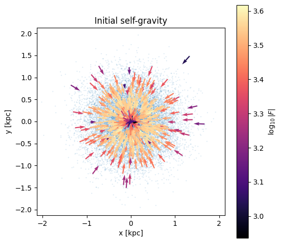
(Executed on a mobile NVIDIA RTX 4070 in my case.) The returned loc object is a LocalExpansion. It stores the local Taylor expansion of the potential evaluated at every particle. loc.force() extracts the corresponding force vectors. Here a tiny visualization of some of the forces:

force = loc.force()
force_norm = jnp.linalg.norm(force, axis=-1)
force_direction = force / jnp.maximum(force_norm[:, None], 1.0e-20)
sample = slice(None, None, 2048)
limit = float(jnp.max(jnp.abs(satellite.pos[::64, :2]))) * 1.05

fig, ax = plt.subplots(figsize=(6, 6))
ax.scatter(satellite.pos[::64, 0], satellite.pos[::64, 1], s=0.3, alpha=0.15)
arrows = ax.quiver(
    satellite.pos[sample, 0], satellite.pos[sample, 1],
    force_direction[sample, 0], force_direction[sample, 1],
    jnp.log10(force_norm[sample]), cmap="magma", angles="xy", scale_units="xy",
    scale=4.0, width=0.006,
)
fig.colorbar(arrows, ax=ax, label=r"$\log_{10}|F|$")
ax.set(xlim=(-limit, limit), ylim=(-limit, limit), xlabel="x [kpc]", ylabel="y [kpc]",
       aspect="equal", title="Initial self-gravity")
plt.show()

Evolve a particle distribution

A default SimConfig combines the FMM force solver with a drift-kick-drift integrator. The array ts contains the initial time and every integration endpoint, while simulate returns the final particle state.

satellite_initial = make_satellite()
cfg_evolution = jzfmm.SimConfig()
satellite_final = jzfmm.time_integration.simulate.jit(
    satellite_initial, ts=jnp.linspace(0.0, 0.01, 41), cfg=cfg_evolution
)

The 3 lines above are really everything that is needed for running a simulation. However, depending on your application, you may be interested in some of the features below.

Snapshots and External Potentials

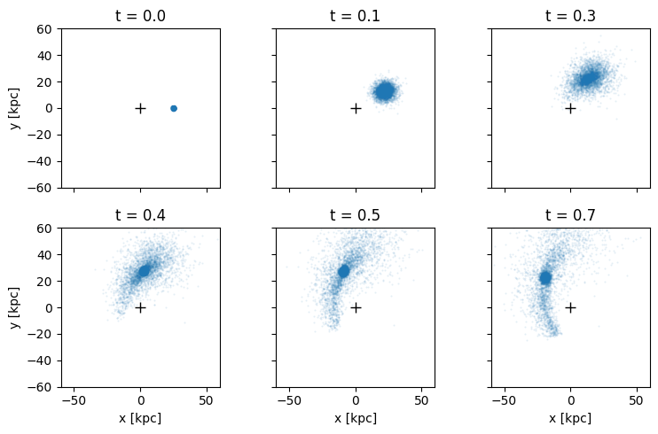
Below you can see how we set up an external Hernquist potential via the config data class. You could easily define your own potentials and they will automatically be differentiated to get forces.

Further, you can see how simulate_with_outputs can be used as a generator for particle outputs. Usually you should process them one by one to not explode the memory (see e.g. hello_world.py), but below we materialize a list that contains all outputs at once for simplicity. simulate_with_outputs should not be jitted, but it calls a jitted simulation function internally.

satellite_orbit = make_satellite(center=(25.0, 0.0, 0.0), bulk_velocity=(0.0, 100.0, 0.0))
cfg_orbit = jzfmm.SimConfig()
cfg_orbit.force.kernel.softening = 0.2
cfg_orbit.external_potential = jzfmm.external_potential.HernquistPotential(
    a=10.0, mass=1.0e11
)

orbit_snapshots = list(jzfmm.time_integration.simulate_with_outputs(
    satellite_orbit, tend=0.8, nout=6, steps_per_output=20, cfg=cfg_orbit
))

[time_integration.py:366] Compiling jitted simulation...
[time_integration.py:379] Compilation done after 2.53s
[time_integration.py:393] Reached output 1 (0.92s for 20 steps)
[time_integration.py:393] Reached output 2 (0.94s for 20 steps)
[time_integration.py:393] Reached output 3 (0.75s for 20 steps)
[time_integration.py:393] Reached output 4 (0.96s for 20 steps)
[time_integration.py:393] Reached output 5 (0.81s for 20 steps)
[time_integration.py:393] Reached output 6 (0.96s for 20 steps)
[time_integration.py:397] Total simulation time: 7.88s for 120 steps

fig, axes = plt.subplots(2, 3, figsize=(8, 5), sharex=True, sharey=True)
for ax, (snapshot_time, state) in zip(axes.flat, orbit_snapshots):
    ax.scatter(state.pos[::64, 0], state.pos[::64, 1], s=0.3, alpha=0.1)
    ax.plot(0.0, 0.0, marker="+", color="black", markersize=8)
    ax.set(title=f"t = {float(snapshot_time):.1f}", aspect="equal")
    ax.set_xlim(-60,60)
    ax.set_ylim(-60,60)
for ax in axes[-1]:
    ax.set_xlabel("x [kpc]")
for ax in axes[:, 0]:
    ax.set_ylabel("y [kpc]")
plt.tight_layout()
plt.show()

Reconstructing a satellite with differentiable simulations

We finish with a small inverse problem based on the disrupting satellite above. Its initial center-of-mass position is now unknown, while its initial center-of-mass velocity is assumed to be known. We generate a target from the same Hernquist-orbit setup and use gradient descent to recover the initial position vector.

A differentiable simulation treats the final particle distribution as a function of its initial conditions. A loss is defined based on the final state. Reverse-mode differentiation propagates its gradient back through every integration step to the initial position.

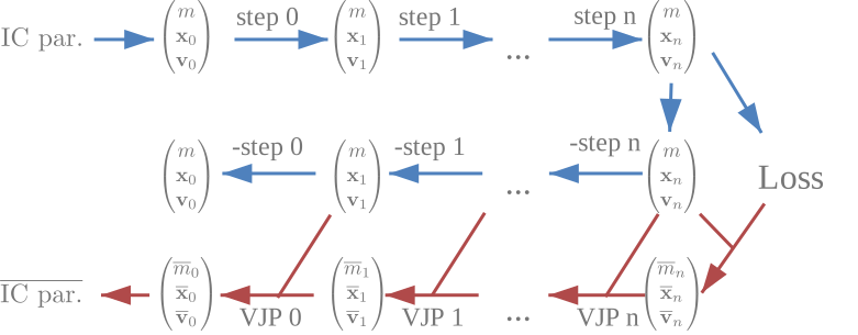
jz-fmm reconstructs earlier particle states during the backward pass instead of retaining the full forward trajectory. We recommend DKDLatticeConfig for this workflow because its integer phase-space updates are perfectly reversible. Its dx and dv parameters are the position and velocity lattice spacings: choose them substantially smaller than the smallest changes that need to be resolved, while ensuring that the full position and velocity range fits into the selected integer dtype. Smaller spacings improve quantization resolution but reduce the available dynamic range. int64 provides considerably more range than int32.

Since we need to run many simulations here, we use a smaller number of 200,000 particles to keep things interactive. Note also that evaluating the gradient of a simulation takes more or less three times as long as just running the simulation, for the reasons mentioned above.

target_com_pos = jnp.array([25.0, 0.0, 0.0])
target_com_vel = jnp.array([0.0, 100.0, 0.0])
ts_reconstruction = jnp.linspace(0.0, 0.8, 21)
satellite_base = make_satellite(nparticles=200_000)
cfg_reconstruction = jzfmm.SimConfig()
cfg_reconstruction.force.kernel.softening = 0.5
cfg_reconstruction.integrator = jzfmm.DKDLatticeConfig(dx=1.0e-5, dv=1.0e-5)
cfg_reconstruction.external_potential = jzfmm.external_potential.HernquistPotential(
    a=10.0, mass=1.0e11
)

target_initial = replace(
    satellite_base,
    pos=satellite_base.pos + target_com_pos,
    vel=satellite_base.vel + target_com_vel,
)
target_final = jzfmm.time_integration.simulate.jit(
    target_initial, ts=ts_reconstruction, cfg=cfg_reconstruction
)

For each proposed COM position vector, we evolve a new initial state and compare its final distribution with the target using the maximum mean discrepancy (MMD) with a distance kernel. This loss is zero if the distributions are identical and grows approximately linearly at large distances. Its diagonal terms require remove_self_interaction=False.

cfg_loss = jzfmm.FMMConfig(
    kernel=jzfmm.SoftenedDistanceKernel(softening=1.0),
    remove_self_interaction=False,
)

def reconstruction_loss(com_pos):
    trial_initial = replace(
        satellite_base,
        pos=satellite_base.pos + com_pos,
        vel=satellite_base.vel + target_com_vel,
    )
    trial_final = jzfmm.time_integration.simulate(
        trial_initial, ts=ts_reconstruction, cfg=cfg_reconstruction
    )
    return jzfmm.loss.maximum_mean_discrepancy(
        trial_final, target_final, cfg_fmm=cfg_loss
    )


loss_and_grad = jax.jit(jax.value_and_grad(reconstruction_loss, argnums=(0, )))

Note that we can differentiate this custom loss function with jax.value_and_grad because all used functions support it. In particular the simulate function implements the custom VJP rule that we have mentioned above. Note that we should wrap our gradient function in jax.jit for performance.

Here, we only optimize the initial position of the object. It is also possible to recover the velocity in these types of problem setups (see the article), but it requires notable numerical care and we want to focus on the code interface here.

com_pos = jnp.array([70.0, 12., -30.])
com_pos_history = []
loss_history = []

print(f"Target COM position:    {target_com_pos}")

for iteration in range(51):
    loss_value, (gradient_pos, ) = loss_and_grad(com_pos)
    com_pos_history.append(com_pos)
    loss_history.append(float(loss_value))
    if iteration % 5 == 0:
        print(f"{iteration:2d}: loss={float(loss_value):.4g}, com_pos={com_pos}")
    com_pos = com_pos - 2.0 * gradient_pos * jnp.exp(-iteration/20.) 


print(f"Recovered COM position: {com_pos}")

Target COM position:    [25.  0.  0.]
 0: loss=182.2, com_pos=[ 70.  12. -30.]
 5: loss=110.5, com_pos=[ 49.893353   -1.0784526 -22.555832 ]
10: loss=19.34, com_pos=[ 28.52592  -10.602045 -12.75319 ]
15: loss=7.04, com_pos=[25.987001 -8.286052 -6.103718]
20: loss=3.07, com_pos=[26.148773  -5.74695   -2.8117695]
25: loss=1.396, com_pos=[25.935814  -3.9480772 -1.2598283]
30: loss=0.6892, com_pos=[25.737083   -2.7650678  -0.60030824]
35: loss=0.376, com_pos=[25.543392  -2.0367284 -0.3194755]
40: loss=0.228, com_pos=[25.44389    -1.5775563  -0.19215903]
45: loss=0.1528, com_pos=[25.366676   -1.2880461  -0.12863967]
50: loss=0.1114, com_pos=[25.315706   -1.0973232  -0.09403995]
Recovered COM position: [25.307571   -1.0674025  -0.08911773]

com_pos_history = jnp.stack(com_pos_history)
fig, axes = plt.subplots(1, 2, figsize=(8, 3.5))
axes[0].plot(loss_history, marker="o")
axes[0].set(xlabel="Gradient step", ylabel="MMD loss", yscale="log")
for component, label in enumerate(("x", "y", "z")):
    axes[1].plot(com_pos_history[:, component], marker="o", label=label)
    axes[1].axhline(target_com_pos[component], color=f"C{component}", linestyle="--")
axes[1].set(xlabel="Gradient step", ylabel="COM position [kpc]")
axes[1].legend(title="Component")
plt.tight_layout()
plt.show()

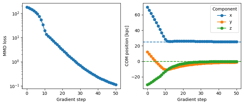
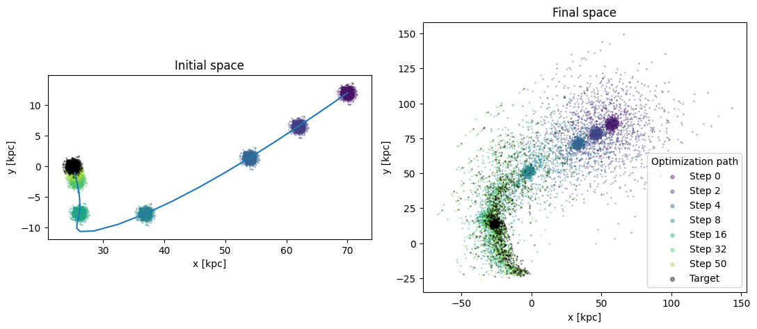
The reconstruction can be refined further by continuing the optimization, but the gradient already brings us close to the target quite rapidly. Below you can see the optimization path. Remember that every step runs its own simulation followed by a backward pass and gradient propagation.

history_indices = [0, 2, 4, 8, 16, 32, 50]
reconstruction_states = []

for index in history_indices:
    initial = replace(
        satellite_base,
        pos=satellite_base.pos + com_pos_history[index],
        vel=satellite_base.vel + target_com_vel,
    )
    final = jzfmm.time_integration.simulate.jit(
        initial, ts=ts_reconstruction, cfg=cfg_reconstruction
    )
    reconstruction_states.append((initial, final))

fig, axes = plt.subplots(1, 2, figsize=(11, 5))
colors = plt.cm.viridis(jnp.linspace(0.05, 0.85, len(history_indices)))
axes[0].plot(com_pos_history[:,0], com_pos_history[:,1])
for color, index, (initial, final) in zip(
    colors, history_indices, reconstruction_states
):
    label = f"Step {index}"
    axes[0].scatter(initial.pos[::100, 0], initial.pos[::100, 1], s=0.5, alpha=0.4,
                    color=color, label=label)
    axes[1].scatter(final.pos[::100, 0], final.pos[::100, 1], s=0.5, alpha=0.4,
                    color=color, label=label)
axes[0].scatter(target_initial.pos[::100, 0], target_initial.pos[::100, 1], s=0.7,
                alpha=0.4, color="black", label="Target")
axes[1].scatter(target_final.pos[::100, 0], target_final.pos[::100, 1], s=0.7,
                alpha=0.4, color="black", label="Target")
for ax, title in zip(axes, ("Initial space", "Final space")):
    ax.set(title=title, xlabel="x [kpc]", ylabel="y [kpc]", aspect="equal")
axes[1].legend(markerscale=5, title="Optimization path")
plt.tight_layout()
plt.show()

Where to go next

The reconstruction above is intentionally simplified. A realistic application should use more particles and time steps, a physically motivated equilibrium profile for the satellite (or even better: cosmological initial conditions), an observationally appropriate loss function, possibly many more degrees of freedom and a better optimization method. As discussed in the article, optimization can be quite tricky in these loss landscapes and needs to be investigated carefully in future work.

The API reference describes the available kernels, integrators, external potentials, and compatibility helpers. For distributed execution, see the multi-GPU guide.

Error handling

Runtime checks inside jitted computations use jz-tree’s host callbacks to raise errors, which can produce long JAX tracebacks with messages such as CpuCallback error. Look for the Relevant Error Message section: it contains the actual cause and often a hint for resolving it. For example, if an interaction list exceeds its allocated capacity, increase the indicated allocation factor in the configuration. See jz-tree’s error-handling section for an example and further explanation.