Tutorial II: Testing Code

How to test numerical code systematically with unit tests.

Posted Oct 8, 2025 Updated Oct 17, 2025

By Jens Stücker

31 min read

Overview

This is the second tutorial of a series about setting up a good workflow for a scientific Python code repository.

Here we will learn how to

Develop robust numerical tests for research code
Set up a unit test system to define easily repeatable tests
Define a healthy test-driven workflow

Prerequisites

I assume that you have gone through the previous tutorial and have set up the spherical-potential code-repository as a starting point.

If you didn’t follow along to set up the repository yourself, you can recreate the starting point for this tutorial by manually creating a fork from the “v0.1” tag of my repository:

  
# Create a new **completely** empty git repository -- e.g. with the name `spherical-potential`
git clone https://github.com/jstuecker/spherical-potential.git
git remote set-url origin <URL-of-your-new-empty-repo>
git switch -C main v0.1   # make your main branch start from v0.1
git push -u origin main

Solving Poisson’s equation

Recall: We want to solve Poisson’s equation in spherical symmetry by solving two integrals. $\begin{align} M(r) &= 4 \pi \int r^2 \rho(r) dr \\ \phi(r) &= G \int \frac{M(r)}{r^2} dr \end{align}$ We already have a function cumulative_integral that evaluates the antiderivative. Let’s add some additional functions that solve these equations to our module file

  
def density_to_mass(rhoi, ri, method="trapezoidal", m0=0.):
    integrand = 4 * np.pi * ri**2 * rhoi
    mi = cumulative_integral(integrand, ri, method=method, initial=m0)
    return mi

def mass_to_potential(mi, ri, G=1., method="trapezoidal", phi0=0.):
    integrand = G * mi / ri**2
    phii = cumulative_integral(integrand, ri, method=method, initial=phi0)
    return phii

def density_to_potential(rhoi, ri, G=1., method="trapezoidal", m0=0., phi0=0.):
    mi = density_to_mass(rhoi, ri, method=method, m0=m0)
    phii = mass_to_potential(mi, ri, G=G, method=method, phi0=phi0)
    return phii

and let’s commit our changes

  
git add src/spherical_potential/integrals.py
git commit -m "Added functions that integrate Poisson's equation in spherical symmetry"
git push # optionally

Note: if we were working on the same repository with multiple people, we should at the very least test that our changes do not break existing code before committing + pushing. We will see later how to cleanly verify our code in advance.

Dimensions of Tests

These functions look plausible, but it is always important to test our code. Making mistakes is very easy… very very easy… Your code will contain bugs and you need to put a bit of effort from time to time to deal with them. The more you accept this and the better you plan for it, the more time you will save and the better you will feel about your code! (Also: the better others will feel about your code!)

There is no one-size-fits-all approach for testing code. What is a good test depends strongly on the objectives and the constraints of your project. So a good first step is to get aware of these. Here, we want to write a code that can solve Poisson’s equation

for a set of known pre-defined profiles
for possibly quite arbitrary user-defined profiles

Further it is good to be aware that code “correctness” may come at different “resolution” levels. E.g. after implementing some new code, we may want to check

that the syntax is valid – e.g. by trying to import the module
that our new function does what it is supposed to do – e.g. by testing for known inputs/outputs (e.g. an analytic solution, a reference implementation or against a higher resolution scenario)
that our function integrates correctly with the rest of our code – e.g. by doing similar tests for other higher level functions that use our function
that our function behaves correctly for a large variety of inputs and outputs – let’s call a corresponding test an input coverage test

Given our very broad objective, it would probably be a good idea to verify our code on all of these levels. Note that e.g. the input coverage test aspect may be less relevant if your code only needs to work for a single scenario. Further, it is sometimes sufficient to test your code only on a higher level (3) and not to test every function individually (2).

When deciding what aspects of your code to test, always take a step back and think a bit about it. And once you have implemented a meaningful test, reward yourself for it – especially if your code doesn’t pass it, since it means that you have found a bug and prevented a lot of potential suffering!

In our scenario it is relatively easy to think of a good way to test our code. We are solving Poisson’s equation numerically, but there are a lot of analytical reference cases available. Testing against these will provide robust and meaningful verification.

Testing for correctness

We have already written a small test for the cumulative_integral function in our notebook. Let us start by creating a similar test for our density_to_mass function, by testing against the Plummer profile

\[\begin{align} \rho(r) &= \frac{3 M_0}{4 \pi a^3} \left(1 + \frac{r^2}{a^2} \right)^{-5/2} \\ M(r) &= M_0 \frac{r^3}{(r^2 + a^2)^{3/2}} \\ \phi(r) &= - \frac{G M_0} {\sqrt{r^2 + a^2}} \end{align}\]

We can bundle the corresponding functions into a class. To keep our code organized, let’s put it into a new file src/spherical_potential/analytical_profiles.py

  
from dataclasses import dataclass
import numpy as np

@dataclass
class PlummerProfile:
    M : float = 1.
    a : float = 1.
    G : float = 1.

    def density(self, r):
        return (3*self.M/(4*np.pi*self.a**3)) * (1 + (r/self.a)**2)**(-5/2)

    def m_of_r(self, r):
        return self.M * r**3 / (r**2 + self.a**2)**(3/2)

    def potential(self, r):
        return -self.G * self.m_of_r(r) / r

If you don’t know what a dataclass is, consider reading about it – dataclasses are awesome! They remove a lot of boilerplate code by defining a default constructor and some other useful methods through a single decorator.

and let’s not forget to include our new submodule in our __init__.py:

  
from . import integrals
from . import analytical_profiles

Let’s verify at least on level 1 and check that we can import and initialize the class – e.g. in our notebook

  
prof = sp.analytical_profiles.PlummerProfile(M=10.)
print(prof)
# outputs: PlummerProfile(M=10.0, a=1.0, G=1.0)

and then commit our changes (by now you know the drill!)

Now let’s test our integrals against our new reference profile

  
prof = sp.analytical_profiles.PlummerProfile(M=10.)

ri = np.logspace(-2, 2, 200)
rho_ana = prof.density(ri)

m_num = sp.integrals.density_to_mass(rho_ana, ri)
m_ana = prof.m_of_r(ri)

phi_num = sp.integrals.mass_to_potential(m_ana, ri)
phi_num_full = sp.integrals.density_to_potential(rho_ana, ri)
phi_ana = prof.potential(ri)

fig, axs = plt.subplots(1, 2, figsize=(10, 5))

axs[0].loglog(ri, prof.m_of_r(ri))
axs[0].loglog(ri, m_num, ls='dashed')
axs[0].set_xlabel('r')
axs[0].set_ylabel('M(<r)')
axs[0].legend(['analytical', 'numerical'])
axs[1].plot(ri, prof.potential(ri), label='analytical')
axs[1].plot(ri, phi_num, ls='dashed', label='numerical (mass_to_potential)')
axs[1].plot(ri, phi_num_full, ls='dotted', label='numerical (density_to_potential)')
axs[1].set_xlabel('r')
axs[1].set_ylabel('Phi(r)')
axs[1].legend()

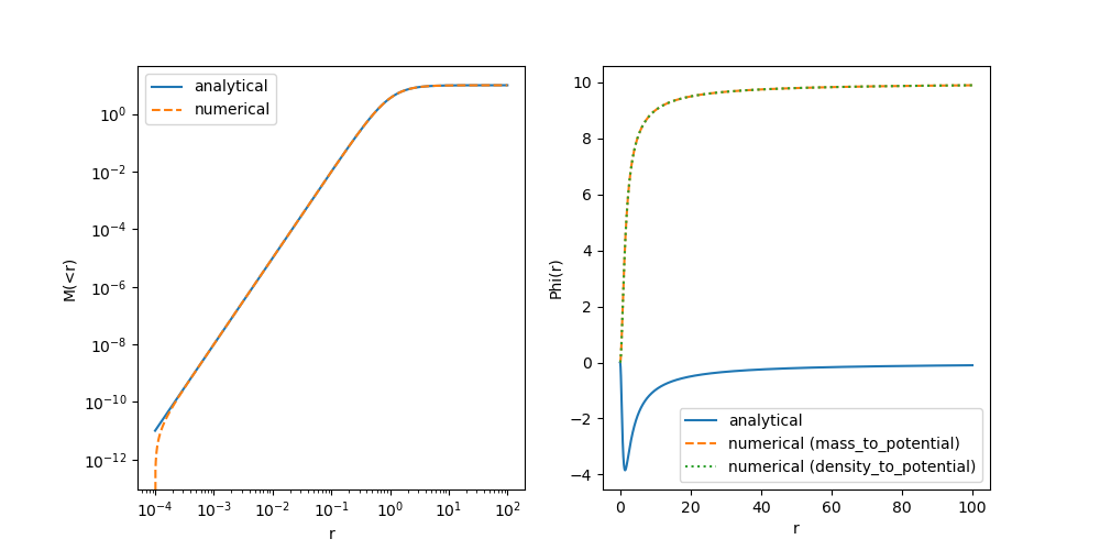
This is odd! The mass profile doesn’t agree at very small radii… and the potential seems wrong everywhere. First, let’s double check that we implemented the Plummer profile correctly…

After some inspection I have found the following mistake:

  
[...]
class PlummerProfile:
    [...]
    # wrong version (this is not a point mass!):
    # def potential(self, r):
    #     return -self.G * self.m_of_r(r) / r
    # corrected version:
    def potential(self, r):
        return -self.G * self.M / np.sqrt(r**2 + self.a**2)

Do you know how I made this mistake? By quickly tabbing through Copilot’s suggested autocompletion for the Plummer profile. Good that we have checked this!

First of all, let’s commit this fix (E.g. with a message like “Fixed an error in the Plummer potential”). And now let’s recheck our plot:

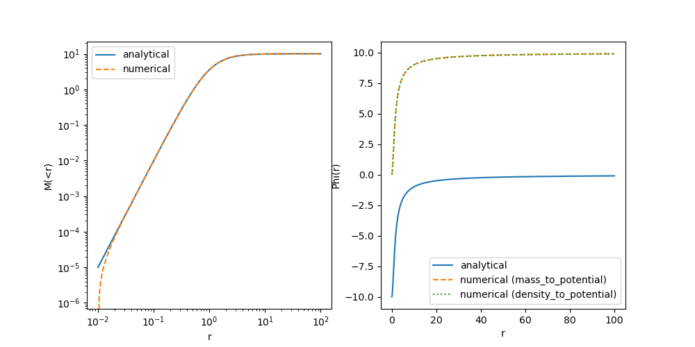
The Potential is still wrong everywhere, but now the reason is much easier to identify. Think about it and only move on once you have a good idea!

Clearly there is a constant offset missing between our profiles! The analytical solution provides a potential that is normalized to $\phi(r \rightarrow \infty) \rightarrow 0$ – i.e. vacuum boundary conditions – whereas we had normalized our numerical solution towards $\phi(r \rightarrow 0) \rightarrow 0$. Arguably both are valid choices (since an offset in the potential does not affect the dynamics), but to stay consistent with the literature, let’s adopt the vacuum boundary conditions.

Let’s correct our code

  
def mass_to_potential(mi, ri, G=1., method="trapezoidal", exterior_potential=0.):
    """
    Compute the gravitational potential from a mass profile assuming spherical symmetry.

    Parameters
    ----------
    mi : array_like
        Mass profile as a function of radius.
    ri : array_like
        Radii corresponding to the mass profile.
    G : float, optional
        Gravitational constant
    method : str, optional
        Integration method. Currently only "trapezoidal" is implemented.
    exterior_potential : float, optional
        Potential at ri[-1] that is sourced by mass from r > ri[-1]. By default, the potential
        will be returned as if no mass exists outside ri[-1].
    """
    integrand = G * mi / ri**2
    phii = cumulative_integral(integrand, ri, method=method, initial=0.)

    phiboundary = -G * mi[-1] / ri[-1]

    return phii + (phiboundary - phii[-1]) + exterior_potential

def density_to_potential(rhoi, ri, G=1., method="trapezoidal", m0=0., exterior_potential=0.):
    mi = density_to_mass(rhoi, ri, method=method, m0=m0)
    phii = mass_to_potential(mi, ri, G=G, method=method, exterior_potential=exterior_potential)
    return phii

Here, we have corrected the normalization by matching it to the one of a point-mass at the outer-most radius. Since there could be additional contributions from the mass distribution at larger radii – which our integrator doesn’t have access to – we also give the user the option to correct for the exterior mass. (For the Plummer potential these are anyway so small that we don’t need to worry about them though.)

We have also added a doc-string here. When publishing a code, it is important to provide a good documentation for most functions. I included this as an example so that you know how to do this. That said, I don’t recommend writing too much documentation while your code is still heavily changing, because it may double your work during development and it may make it more difficult to focus on what is important. However, since exterior_potential is a rather confusing parameter, it is good to write down its meaning somewhere, so that we do not forget about it. In practice, I’d just document that parameter in the docstring during development and then later complete the documentation when I am about to publish my code.

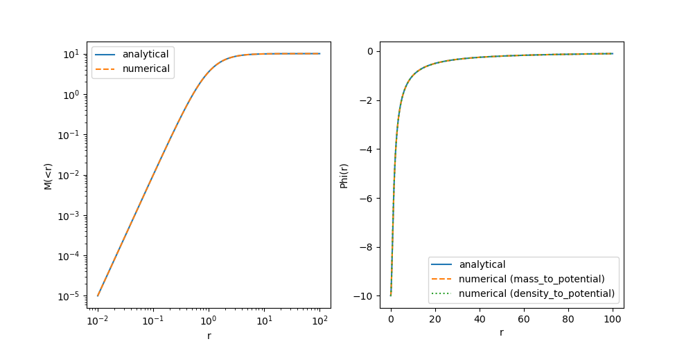
Now let’s run the test again in our notebook. You can see that the potential is matching quite well now! The mass-profile is still a bit off at small radii. At this point, you probably have a good idea what might be needed to correct this.

💡 Show solution

We need to pass the mass that is at radii < ri[0] to our functions, since our integration code also does not know the boundary conditions for the mass-profile at r < r[0]

  
[...]
m_num = sp.integrals.density_to_mass(rho_ana, ri, m0=prof.m_of_r(ri[0]))
[...]
phi_num_full = sp.integrals.density_to_potential(rho_ana, ri, m0=prof.m_of_r(ri[0]))
[...]

With this, we get a very good match! As usual, let’s commit our code with the new corrections.

Awesome! We have created a little test and we have verified our new code at level 1-3 as discussed earlier. We can be sure now that our newly written function does what we want it to do – at least for a single test case. I hope you agree, that this is something we should always do when writing new code.

In principle we could now move on, write more code, add more tests into our notebook etc… This would already be a reasonable workflow. However, here are some aspects that are not totally optimal with that:

The two tests that we have already created are actually quite different and rather independent from each other… why would we want to keep them in a linear file – maybe they should have their own dedicated place…?
It may happen in the future that we want to change some aspect of our code that could invalidate our tests (E.g. imagine we change the integrator in our cumulative_integral function)
- In that case we should rerun the tests… but imagine we have 10s or 100s of tests for our code and we’d have to dig through all of our notebooks to find them… possibly we wouldn’t even remember which things may have been affected by our change
- It may happen that we make a change and we are completely unaware that it invalidates something that we have established to work earlier.
If we are working together with others, they probably do not know which test we have put where in which notebook and why, It would be very difficult for them to redo our tests without detailed instruction…

–> Wouldn’t it be great, to set up a system where we or anyone else can easily repeat all of our tests with minimal effort?

Well… we have just reinvented “unit tests”! It is actually really simple to set up such a system of tests and it is also very rewarding. Trust me, once you get used to it a bit, it will cost you almost zero extra time to convert your tests into reproducible unit tests!

In particular, unit tests will allow us to

Easily rerun all of our tests every time when we change some code or before we commit our changes
Immediately detect if we made a change that did break something that breaks earlier code.
Be braver when we need to make a change that affects all of our code-base.
Feel good about our code

Setting up unit tests

Working with unit tests is a lot more fun from VSCode than from the command line. However, as usual, it is good to first know what is happening under the hood before you use a more convenient graphical interface. Let’s get started by installing pytest

pip install pytest

and by creating a directory called tests with a file tests/test_potential.py.

pytest has a strict naming convention for unit tests. Each file that contains unit tests either has to start with “test_” or has to end with “_test.py”. A similar requirement holds for the names of functions that execute unit tests.

Right now my directory has the following structure:

  
tree --noreport -I '.git'
.
├── LICENSE
├── README.md
├── notebooks
│   └── potentials.ipynb
├── pyproject.toml
├── src
│   ├── spherical_potential
│   │   ├── __init__.py
│   │   ├── analytical_profiles.py
│   │   └── integrals.py
└── tests
    └── test_integrals.py

Let’s write our first unit test:

  
def test_that_passes():
    assert True

(I told you it wouldn’t be so difficult.) Running the test is also very simple. From the repository’s root directory do:

pytest -v

(pytest will auto locate your test scripts by the “test” naming convention) or if you want to be unnecessarily precise you can also execute like this

  
pytest tests -v
# or
pytest tests/test_integrals.py -v

You should see an output similar to this, confirming that our test passed:

    ============================= test session starts ==============================
    platform linux -- Python 3.12.11, pytest-8.4.2, pluggy-1.6.0 -- /home/jens/repos/spherical-potential/.venv/bin/python3
    cachedir: .pytest_cache
    rootdir: /home/jens/repos/spherical-potential
    configfile: pyproject.toml
    collecting ... collected 1 item

    tests/test_integrals.py::test_that_passes PASSED                         [100%]

    ============================== 1 passed in 0.01s ===============================

Let’s make this more interesting with a few more “tests”:

  
def test_that_passes():
    assert True

def test_also_passes():
    print("I am trying to print something, but no one will see it :(")
    assert True

def test_that_fails():
    assert False

and let’s run it:

============================= test session starts ==============================
platform linux -- Python 3.12.11, pytest-8.4.2, pluggy-1.6.0 -- /home/jens/repos/spherical-potential/.venv/bin/python3
cachedir: .pytest_cache
rootdir: /home/jens/repos/spherical-potential
configfile: pyproject.toml
collecting ... collected 3 items

tests/test_integrals.py::test_that_passes PASSED                         [ 33%]
tests/test_integrals.py::test_that_fails FAILED                          [ 66%]
tests/test_integrals.py::test_also_passes PASSED                         [100%]

=================================== FAILURES ===================================
_______________________________ test_that_fails ________________________________

    def test_that_fails():
>       assert False
E       assert False

tests/test_integrals.py:5: AssertionError
=========================== short test summary info ============================
FAILED tests/test_integrals.py::test_that_fails - assert False
========================= 1 failed, 2 passed in 0.04s ==========================

Note how pytest first runs all the tests and then informs us afterwards of the tests that have failed, including an indication of the precise line from which the error was raised.

pytest has by default a very compressed output, since it is intended to scale towards very large test suites. We are already using the verbose “-v” option that gives a bit more information about the tests that have passed, but we still do not see the output of our print statement. To see the output of our scripts, you additionally have to use “-s”, as in pytest -v -s

At this point you know everything essential about how unit tests operate. Now we just need a meaningful example, but before we go there, let’s discuss briefly how to set up unit tests with VSCode:

Unit Tests with VSCode

Consider having a look at this guide. In short: You need to click the “Testing” button on the left, then you press “Configure Python Test”, select “pytest” and select the “tests” directory. That’s it!

You may note that VSCode has created a file .vscode/settings.json with some configuration options. I recommend also adding --color=yes to “python.testing.pytestArgs”. Commit this file to the repository together with our dummy unit test. This way you won’t have to configure VSCode again if you clone the repository on another machine.

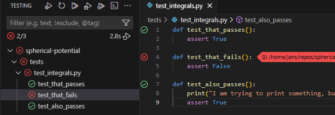
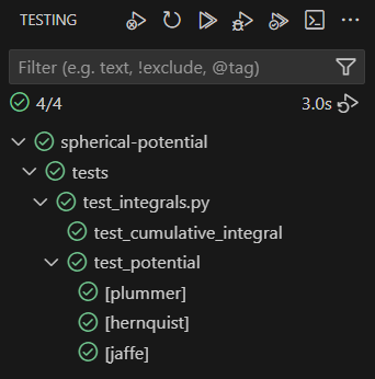
You should now see an overview of the tests in the side-bar. You can run them all at once or you can run each individually by hovering over the test and clicking the “run” arrow button.

Another very useful feature is the “run and debug” button just next to the “run” button. This runs the debugger for a particular unit test (e.g. allowing you to stop execution at custom break-points). If you want the debugger to spawn when an error is raised (which generally you do), go to “Run and Debug” and check the “Raised Exceptions” Breakpoint in the bottom left. Debugging your code interactively can be extremely useful and it might be a good topic for a future tutorial. Unit tests give you very convenient entry points for debugging interactively.

After running your tests you should see a nice overview of things that worked and didn’t work, just as we did when running pytest from the command line, but it is much easier e.g. to repeat tests selectively.

Our first unit test

Delete our dummy unit tests and let us create a meaningful one based on the test of cumulative_integral from our notebook:

  
import numpy as np
import spherical_potential as sp

def test_cumulative_integral():
    x = np.linspace(0, 10, 100)
    y = sp.integrals.cumulative_integral(x**2, x)

    assert np.allclose(y, x**3 / 3, atol=1e-2)

collecting ... collected 1 item

tests/test_integrals.py::test_cumulative_integral FAILED                 [100%]

=================================== FAILURES ===================================
___________________________ test_cumulative_integral ___________________________

    def test_cumulative_integral():
        x = np.linspace(0, 10, 100)
        y = sp.integrals.cumulative_integral(x**2, x)
    
>       assert np.allclose(y, x**3 / 3, atol=1e-2)
E       assert False
E        +  where False = <function allclose at 0x781dfa595e30>(array([0.00000000e+00, 5.15305076e-04, 3.09183046e-03, 9.79079645e-03,\n       2.26734233e-02, 4.38009315e-02, 7.52345411e-02, 1.19035473e-01,\n       1.77264946e-01, 2.51984182e-01, 3.45254401e-01, 4.59136823e-01,\n       5.95692668e-01, 7.56983157e-01, 9.45069510e-01, 1.16201295e+00,\n       1.40987469e+00, 1.69071595e+00, 2.00659797e+00, 2.35958194e+00,\n       2.75172911e+00, 3.18510068e+00, 3.66175787e+00, 4.18376191e+00,\n       4.75317402e+00, 5.37205542e+00, 6.04246732e+00, 6.76647095e+00,\n       7.54612753e+00, 8.38349828e+00, 9.28064442e+00, 1.02396272e+01,\n       1.12625077e+01, 1.23513474e+01, 1.35082073e+01, 1.47351487e+01,\n       1.60342327e+01, 1.74075208e+01, 1.88570740e+01, 2.03849535e+01,\n       2.19932206e+01, 2.36839366e+01, 2.54591626e+01, 2.73209598e+01,\n       2.92713895e+01, 3.13125129e+01, 3.34463913e+01, 3.56750857e+01,\n       3.80006575e+01, 4.04251679e+01, 4.29506781e+01, 4.55792493e+01,\n       4.83129427e+01, 5.11538196e+01, 5.41039412e+01, 5.71653686e+01,\n       6.03401632e+01, 6.36303861e+01, 6.70380986e+01, 7.05653618e+01,\n       7.42142371e+01, 7.79867855e+01, 8.18850684e+01, 8.59111470e+01,\n       9.00670824e+01, 9.43549360e+01, 9.87767688e+01, 1.03334642e+02,\n       1.08030617e+02, 1.12866756e+02, 1.17845118e+02, 1.22967766e+02,\n       1.28236760e+02, 1.33654162e+02, 1.39222034e+02, 1.44942435e+02,\n       1.50817428e+02, 1.56849074e+02, 1.63039434e+02, 1.69390569e+02,\n       1.75904541e+02, 1.82583410e+02, 1.89429238e+02, 1.96444086e+02,\n       2.03630015e+02, 2.10989087e+02, 2.18523362e+02, 2.26234903e+02,\n       2.34125769e+02, 2.42198023e+02, 2.50453726e+02, 2.58894939e+02,\n       2.67523722e+02, 2.76342138e+02, 2.85352247e+02, 2.94556111e+02,\n       3.03955791e+02, 3.13553348e+02, 3.23350843e+02, 3.33350338e+02]), ((array([ 0.        ,  0.1010101 ,  0.2020202 ,  0.3030303 ,  0.4040404 ,\n        0.50505051,  0.60606061,  0.70707071,  0.80808081,  0.90909091,\n        1.01010101,  1.11111111,  1.21212121,  1.31313131,  1.41414141,\n        1.51515152,  1.61616162,  1.71717172,  1.81818182,  1.91919192,\n        2.02020202,  2.12121212,  2.22222222,  2.32323232,  2.42424242,\n        2.52525253,  2.62626263,  2.72727273,  2.82828283,  2.92929293,\n        3.03030303,  3.13131313,  3.23232323,  3.33333333,  3.43434343,\n        3.53535354,  3.63636364,  3.73737374,  3.83838384,  3.93939394,\n        4.04040404,  4.14141414,  4.24242424,  4.34343434,  4.44444444,\n        4.54545455,  4.64646465,  4.74747475,  4.84848485,  4.94949495,\n        5.05050505,  5.15151515,  5.25252525,  5.35353535,  5.45454545,\n        5.55555556,  5.65656566,  5.75757576,  5.85858586,  5.95959596,\n        6.06060606,  6.16161616,  6.26262626,  6.36363636,  6.46464646,\n        6.56565657,  6.66666667,  6.76767677,  6.86868687,  6.96969697,\n        7.07070707,  7.17171717,  7.27272727,  7.37373737,  7.47474747,\n        7.57575758,  7.67676768,  7.77777778,  7.87878788,  7.97979798,\n        8.08080808,  8.18181818,  8.28282828,  8.38383838,  8.48484848,\n        8.58585859,  8.68686869,  8.78787879,  8.88888889,  8.98989899,\n        9.09090909,  9.19191919,  9.29292929,  9.39393939,  9.49494949,\n        9.5959596 ,  9.6969697 ,  9.7979798 ,  9.8989899 , 10.        ]) ** 3) / 3), atol=0.01)
E        +    where <function allclose at 0x781dfa595e30> = np.allclose

tests/test_integrals.py:8: AssertionError
=========================== short test summary info ============================
FAILED tests/test_integrals.py::test_cumulative_integral - assert False
============================== 1 failed in 0.11s ===============================

You can see that our test fails, because our integrator doesn’t achieve the $10^{-2}$ absolute accuracy that we test for with np.allclose. Pytest gives us some nicer ways to compare arrays with meaningful error messages:

  
import numpy as np
import spherical_potential as sp
import pytest

def test_cumulative_integral():
    x = np.linspace(0, 10, 100)
    y = sp.integrals.cumulative_integral(x**2, x)

    assert y == pytest.approx(x**3 / 3, abs=1e-2)

============================= test session starts ==============================
platform linux -- Python 3.12.11, pytest-8.4.2, pluggy-1.6.0 -- /home/jens/repos/spherical-potential/.venv/bin/python3
cachedir: .pytest_cache
rootdir: /home/jens/repos/spherical-potential
configfile: pyproject.toml
collecting ... collected 1 item

tests/test_integrals.py::test_cumulative_integral FAILED                 [100%]

=================================== FAILURES ===================================
___________________________ test_cumulative_integral ___________________________

    def test_cumulative_integral():
        x = np.linspace(0, 10, 100)
        y = sp.integrals.cumulative_integral(x**2, x)
    
>       assert y == pytest.approx(x**3 / 3, abs=1e-2)
E       AssertionError: assert array([0.0000...33350338e+02]) == approx([0.0 ±...33333 ± 0.01])
E         
E         comparison failed. Mismatched elements: 41 / 100:
E         Max absolute difference: 0.017005067510126537
E         Max relative difference: 0.00014361625736035227
E         Index | Obtained           | Expected                 
E         (59,) | 70.56536181115305  | 70.55522747799046 ± 0.01 
E         (60,) | 74.21423705476353  | 74.20393095324225 ± 0.01 ...
E         
E         ...Full output truncated (39 lines hidden), use '-vv' to show

tests/test_integrals.py:9: AssertionError
=========================== short test summary info ============================
FAILED tests/test_integrals.py::test_cumulative_integral - AssertionError: assert array([0.0000...33350338e+02]) == approx([0.0 ±...33...
============================== 1 failed in 0.10s ===============================

(Another good alternative is to use numpys method np.testing.assert_allclose(y, x**3 / 3, atol=1e-2) – a matter of taste.) Clearly this is a much more useful error message! We see that our integrator is doing actually pretty well, with a relative error of $1.4 \cdot 10^{-4}$ among the elements that have an absolute error bigger than 0.01. Asking for a small absolute error for large values like 70 is probably not very reasonable. Let us update the test with a relative error bound:

  
assert y == pytest.approx(x**3 / 3, rel=1e-3, abs=1e-2)

This test will only fail when both the absolute error is larger than $10^{-2}$ and the relative is larger than $10^{-3}$. E.g. try once using only the relative bound and you will find the test to fail close to zero – where it becomes not ideal to require a relative error bound.

Now that we have a meaningful test, let us commit it. Also let us this test from our notebook – we don’t really need it anymore.

You might disagree here and point out that the code in our notebook additionally plots these functions and therefore it is valuable to keep it – for example to show that your code works to others. In my opinion the test also achieves this and I really like to keep my notebooks as simple as possible so that I can focus well. If I ever need this plot again I can recreate it easily by looking it up in the history of my repository or by copying the test and adding a few lines to plot it. This is a matter of taste, so do whichever you prefer!

Now let us convert our plummer potential test into a unit test. I recommend that you try it yourself before looking up my solution below!

💡 Show solution

  
def test_plummer_potential():
    prof = sp.analytical_profiles.PlummerProfile(M=10.)

    ri = np.logspace(-2, 2, 200)
    rho_ana = prof.density(ri)

    m_num = sp.integrals.density_to_mass(rho_ana, ri, m0=prof.m_of_r(ri[0]))
    m_ana = prof.m_of_r(ri)

    phi_num = sp.integrals.mass_to_potential(m_ana, ri)
    phi_num_full = sp.integrals.density_to_potential(rho_ana, ri, m0=prof.m_of_r(ri[0]))
    phi_ana = prof.potential(ri)

    assert m_num == pytest.approx(m_ana, rel=1e-3)
    assert phi_num == pytest.approx(phi_ana, rel=1e-2)
    assert phi_num_full == pytest.approx(phi_ana, rel=1e-2)

One recommendation: it is a good idea to start with a relative tolerance first and only add a problem specific absolute tolerance if there is a meaningless error caused by a zero-crossing. Here there isn’t, so we don’t need it. If we had passed “atol=1e-2”, then we’d effectively not be testing our mass profile at small radii “r < 0.1”.

============================= test session starts ==============================
platform linux -- Python 3.12.11, pytest-8.4.2, pluggy-1.6.0 -- /home/jens/repos/spherical-potential/.venv/bin/python3
cachedir: .pytest_cache
rootdir: /home/jens/repos/spherical-potential
configfile: pyproject.toml
collecting ... collected 2 items

tests/test_integrals.py::test_cumulative_integral PASSED                 [ 50%]
tests/test_integrals.py::test_plummer_potential PASSED                   [100%]

============================== 2 passed in 0.09s ===============================

I hope you are also starting to feel good about this! Don’t forget to commit!

Input coverage tests

As discussed earlier, it would be great to also test our code on level 4 – i.e. check for a few different profiles whether our integrator is working. For example, it might be that things work out fine for the finite central density Plummer profile, but they don’t for a Hernquist profile with a central singularity. Let’s add the analytical solution for the Hernquist… and while we are at it, let’s also add a Jaffe profile:

  
from dataclasses import dataclass
import numpy as np

class AnalyticalProfile:
    def density(self, r):
        raise NotImplementedError

    def m_of_r(self, r):
        raise NotImplementedError

    def potential(self, r):
        raise NotImplementedError

@dataclass
class PlummerProfile(AnalyticalProfile):
    """Implementation of a Plummer (1911) profile
    
    see: https://en.wikipedia.org/wiki/Plummer_model
    """
    M : float = 1.
    a : float = 1.
    G : float = 1.

    def density(self, r):
        return (3*self.M/(4*np.pi*self.a**3)) * (1 + (r/self.a)**2)**(-5/2)

    def m_of_r(self, r):
        return self.M * r**3 / (r**2 + self.a**2)**(3/2)

    def potential(self, r):
        return -self.G * self.M / np.sqrt(r**2 + self.a**2)

@dataclass
class HernquistProfile(AnalyticalProfile):
    """Implementation of a Hernquist (1990) profile
    
    see:(https://ui.adsabs.harvard.edu/abs/1990ApJ...356..359H/abstract)
    """
    M : float = 1.
    a : float = 1.
    G : float = 1.

    def density(self, r):
        return (self.M/(2*np.pi)) * (self.a / (r * (r + self.a)**3))

    def m_of_r(self, r):
        return self.M * r**2 / (r + self.a)**2

    def potential(self, r):
        return -self.G * self.M / (r + self.a)

@dataclass
class JaffeProfile(AnalyticalProfile):
    """Implementation of a Jaffe (1983) profile
    
    see: https://ui.adsabs.harvard.edu/abs/1983MNRAS.202..995J/abstract
    """
    M : float = 1.
    a : float = 1.
    G : float = 1.

    def density(self, r):
        return (self.M/(4*np.pi)) * (self.a / (r**2 * (r + self.a)**2))

    def m_of_r(self, r):
        return self.M * r / (r + self.a)

    def potential(self, r):
        return self.G * self.M / self.a * np.log(r / (r + self.a))

We also defined a base class that PlummerProfile, HernquistProfile and JaffeProfile inherit from, so that there is a well defined interface that is identical between them.

First run the tests (so we know that we didn’t break previous code) and then commit the changes.

Now let’s add the new profiles to our unit tests. You might be tempted to copy the previous code and make some small modifications, similar to this:

  
def test_hernquist_potential():
    prof = sp.analytical_profiles.HernquistProfile(M=10.)

    ri = np.logspace(-2, 2, 200)
    rho_ana = prof.density(ri)

    m_num = sp.integrals.density_to_mass(rho_ana, ri, m0=prof.m_of_r(ri[0]))
    m_ana = prof.m_of_r(ri)

    phi_num = sp.integrals.mass_to_potential(m_ana, ri)
    phi_num_full = sp.integrals.density_to_potential(rho_ana, ri, m0=prof.m_of_r(ri[0]))
    phi_ana = prof.potential(ri)

    assert m_num == pytest.approx(m_ana, rel=1e-3)
    assert phi_num == pytest.approx(phi_ana, rel=1e-2)
    assert phi_num_full == pytest.approx(phi_ana, rel=1e-2)

This would be fine, but since we might add many more profiles later, it will quickly explode the size of our code. Again, pytest has a very nice feature pytest.mark.parametrize to group several tests with small parametric changes:

  
def get_profile(name):
    if name == "plummer":
        return sp.analytical_profiles.PlummerProfile(M=10.)
    elif name == "hernquist":
        return sp.analytical_profiles.HernquistProfile(M=10.)
    elif name == "jaffe":
        return sp.analytical_profiles.JaffeProfile()
    else:
        raise ValueError(f"Unknown profile: {name}")

@pytest.mark.parametrize("profile", ["plummer", "hernquist", "jaffe"])
def test_potential(profile):
    prof = get_profile(profile)

    ri = np.logspace(-2, 2, 200)
    rho_ana = prof.density(ri)

    m_num = sp.integrals.density_to_mass(rho_ana, ri, m0=prof.m_of_r(ri[0]))
    m_ana = prof.m_of_r(ri)

    phi_num = sp.integrals.mass_to_potential(m_ana, ri)
    phi_num_full = sp.integrals.density_to_potential(rho_ana, ri, m0=prof.m_of_r(ri[0]))
    phi_ana = prof.potential(ri)

    assert m_num == pytest.approx(m_ana, rel=1e-3)
    assert phi_num == pytest.approx(phi_ana, rel=1e-2)
    assert phi_num_full == pytest.approx(phi_ana, rel=1e-2)

When you run the test, you will see the following

============================= test session starts ==============================
platform linux -- Python 3.12.11, pytest-8.4.2, pluggy-1.6.0 -- /home/jens/repos/spherical-potential/.venv/bin/python3
cachedir: .pytest_cache
rootdir: /home/jens/repos/spherical-potential
configfile: pyproject.toml
collecting ... collected 4 items

tests/test_integrals.py::test_cumulative_integral PASSED                 [ 25%]
tests/test_integrals.py::test_potential[plummer] PASSED                  [ 50%]
tests/test_integrals.py::test_potential[hernquist] PASSED                [ 75%]
tests/test_integrals.py::test_potential[jaffe] PASSED                    [100%]

============================== 4 passed in 0.08s ===============================

Note how each different “profile” parameter is treated as its own test. It feels good to know that everything works well!

Unit tests – the payoff

By now you understand quite well how to write and execute unit tests. However, you might still be wondering how and why we might actually save time by defining these tests upfront.

Examples in tutorials are always somewhat artificial. Good practices really only start to make a big difference in very complex situations, but we still have a relatively simple one here… I’ll try my best to get this point across:

Example 1, code simplification

At a later point we realize that it was quite unnecessary to implement our own trapezoidal rule, since there exists already one in the scipy library. We simplify our code:

  
import numpy as np
from scipy.integrate import cumulative_trapezoid

def cumulative_integral(fi, xi, method="trapezoidal", initial=0):
    assert method in ("trapezoidal", ), "Only 'trapezoidal' method is implemented."
    
    return cumulative_trapezoid(fi, x=xi, initial=0.)

If you rerun the unit-tests with this, you immediately notice that something is wrong! If we recreated our original plot with this code, we’d have to pay close attention to spot that there is a mistake here. Probably, we’d just move past this and a lot later we’d start to feel that something became slightly off… with no clue about how this started.

By rerunning our unit tests we detect such mistakes immediately. Once we know that this change contains an error it shouldn’t be difficult to figure out that we handled the initial value wrongly. Here the corrected version:

  
def cumulative_integral(fi, xi, method="trapezoidal", initial=0):
    assert method in ("trapezoidal", ), "Only 'trapezoidal' method is implemented."
    
    return cumulative_trapezoid(fi, x=xi, initial=0.) + initial

(This code looks a bit funny, because SciPy’s cumulative_trapezoid oddly only accepts initial = 0 or None, don’t ask me why…)

Let’s test and then commit the corrected and code!

Example 2, code extension

Much deeper into our project we realize that we need to improve the performance and/or accuracy of our code. For this we want to consider a higher order integrator. The natural next step would be to use Simpson’s rule. Here our code with the new integrator:

  
import numpy as np
from scipy.integrate import cumulative_trapezoid, cumulative_simpson

def cumulative_integral(fi, xi, method="trapezoidal", initial=0):
    if method == "trapezoidal":
        return cumulative_trapezoid(fi, x=xi, initial=0.) + initial
    elif method == "simpson":
        return cumulative_simpson(fi, x=xi, initial=0.) + initial
    else:
        raise ValueError(f"Unknown method: {method}")

We check whether this gives us an improvement for our PlummerProfile and it looks pretty good:

  
prof = sp.analytical_profiles.PlummerProfile(M=10.)

plt.figure(figsize=(6,4))
for N in 50, 100, 200:
    ri = np.logspace(-2, 2, N)
    phi_ana = prof.potential(ri)

    def rel_error(y1, y2):
        return np.abs((y1 - y2) / y2)

    phi_trap = sp.integrals.density_to_potential(prof.density(ri), ri, method="trapezoidal", m0=prof.m_of_r(ri[0]))
    phi_simps = sp.integrals.density_to_potential(prof.density(ri), ri, method="simpson", m0=prof.m_of_r(ri[0]))
    p = plt.loglog(ri, rel_error(phi_trap, phi_ana), label='trapezoidal, N={}'.format(N))
    plt.loglog(ri, rel_error(phi_simps, phi_ana), label='simpson, N={}'.format(N), ls="dashed", color=p[0].get_color())
plt.legend()
plt.xlabel("r")
plt.ylabel("relative error")

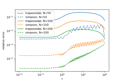
Since Simpsons’s rule apparently only gives us benefits and no drawbacks, we are tempted here to make it our default integrator. At this point, usually, I’d be very nervous of making such a big change. Consider that all of our code depends on our integration rule. E.g. we might worry that for well behaved profiles the higher order integration rule improves our results, but for singular ones like the Hernquist or Jaffe models it might make things worse… If we didn’t standardize our tests, we’d have to redo every check that we have done before to be sure about this, since all of their results may change. Our project is still small right now, but imagine that you had already build a lot more code that depends on this.

All these worries don’t exist when we already have a good set of unit tests! We simply switch the default argument method="trapezoidal" to method="simpson" in all our functions in src/spherical_potential/integrals.py and we rerun our unit tests:

Phew… peace of mind! Let’s commit and go celebrate!

Summary

Testing your code is one of the most important aspects of programming. Some extremists would even argue for creating tests already before writing your code. Getting good at testing is key for writing good code – especially with large language models getting better and better at producing code at an incomprehensible rate.

“Unit tests” are simply a systematic way of managing and rerunning your tests. Obviously they are not a magic solution to all problems you may ever have, but they can improve some aspects of your worflow significantly.

Doing unit tests means to

define some repeatable standardized tests
catch many bugs at the moment they are created
easily prove to others that your code works
make major code changes with cognitive ease
feel good about your code

Obviously you shold only write tests that you consider meaningful. E.g. don’t fall into the trap of worrying about how to measure your code coverage and how to test every last centimeter of your code. I’d simply recommend that whenever you have written a good test, spend a few extra minutes and interface it with pytest. It will be worth it!

You can find a brief overview of useful commands and setup in this cheat sheet.

Tutorials, Python

This post is licensed under CC BY 4.0 by the author.