Tutorial I: Creating a Python Repository

Overview

This is the first tutorial of a series about setting up a good worflow for a scientific python code repository.

This tutorial will cover how to:

• Create a GitHub python repository
• Structure the repository as an installable module, consistent with recent python standards
• Set up a healthy workflow for jupyter notebooks
• Interface this well with VSCode (optionally)

This covers the necessary setup that we will need for the second tutorial where we will learn how to

• Develop robust numerical tests for research code
• Set up a unit test system to define easily repeatable tests
• Define a healthy test-driven workflow

At some point I might consider to create a third tutorial on how to

• Use interactive debuggers to quickly find bugs

To motivate our choices, we will work towards a close-to-real-world example: we will create a python library that solves Poisson’s equation in spherical symmetry for arbitrary spherically symmetric density profiles called spherical-potential.

Prerequisites

I assume that you already understand to some degree how to use

• python
• numpy
• pip
• git

If you don’t know git yet, that is fine, you can still go through this tutorial, but it may be beneficial to consider one of the numerous online resources on git if you don’t understand something. E.g. here are two tutorials for git in general and for git with VSCode

Further, I recommend downloading and working with VSCode. This is optional, but it makes many of the steps easier, since it is well integrated with git and with pytest, works easily on any operating system and does a very good job at code-highlighting and code-completion.

Creating a GitHub repository

Here we set up a code repository on GitHub. GitHub is a very popular site for managing and publishing your code and it interfaces very well with VSCode. However, you could also consider hosting your repository on other sites, like Bitbucket or on a GitLab that is provided by your institute.

• Create a GitHub account (if you haven’t already)
• Create a new repository
  • Repository name: for this tutorial we will go with spherical-potential, but in general you will choose something that is descriptive of your code. You can change this name later on GitHub. It is a good practice to name the repository in a way that is consistent with how you want to import the python library later. For example, we aim to import our code later as import spherical_potential as sp
  • Visibility: We will go with “private” for the start. You can easily change this later
  • Add README: sure, why not
  • Add .gitignore: select “Python”. This will help you to not commit unnecessary files to the repository
  • Add license: If you don’t have a strong opinion on the license, I recommend using the “MIT License”. It basically says “do whatever you want with my code, just don’t sue me”
  • press “Create Repository”
  • Your repository is now accessible over https://github.com/USERNAME/spherical-potential
• Clone the repository
  • If you want to use VSCode:
    • Open a new Window
    • If you are using WSL or if you want to work on a remote machine: press on the bottom left the blue button and establish a connection (e.g. via ssh) – this may require some authentication setup.
    • click: “Clone Git Repository” -> “Clone from GitHub”
    • select your repository name e.g. for me it is “jstuecker/spherical-potential”
    • At some point of this process it may be necessary that you log into your GitHub Account
    • Select a directory where to clone to. I tend to have a directory called “repos” in my home-folder where I keep all my repositories.
  • If you want to go with the command line:

    •   git clone git@github.com:jstuecker/spherical-potential.git
      

    • It may be necessary that you set up a proper SSH authentication by generating a SSH key, registering it on your system and on GitHub. It is described here, how to do this.

Standard python library structure

A good standard directory layout to follow in python libraries is the following:

├── README.md
├── LICENSE
├── pyproject.toml
├── src/
│    └── spherical_potential/
│       ├── __init__.py
│       └── fileA.py
        └── fileB.py

Additional directories that include e.g. notebooks or unit tests may be added to the root directory level and will not be part of the importable package. E.g.

├── README.md
├── LICENSE
├── pyproject.toml
├── src/
│    └── spherical_potential/
│       ├── __init__.py
│       └── fileA.py
|       └── fileB.py
├── notebooks/
│    └── mynotebook.ipynb
|    └── ...
├── tests/
│    └── test_accuracy.py
│    └── ...

Here we will work towards such a structure step-by-step.

Starting with a jupyter notebook

Let us begin with a simple jupyter notebook. Notebooks are great starting points for a code-project, but it is important to be aware of their pros and cons:

✅ Pros — great for exploration

• Immediate feedback loop; run a cell, see results right away.
• Code + narrative + plots in one place; perfect for teaching and EDA.
• Easy to try ideas, tweak parameters, and visualize quickly.
• Shareable (HTML/PDF) and demo-friendly.

⚠️ Cons — long-term: fragile code infrastructure

• Hidden state & out-of-order execution can break reproducibility.
• Harder to review, test, and refactor than plain .py modules.
• Files may become very large so that keeping them under version control may become difficult
• Code cannot be reused across different files

Recommended Workflow

• Use notebooks to prototype, develop tests and explain.
• As code stabilizes, extract logic into src/ python files (functions/classes), import them back into the notebook for plots and narrative.
• Extract tests into dedicated unit tests
• Keep notebooks thin: parameters, visuals, and prose; keep logic in .py with tests.
• Set up with nbstripout to keep commits small

I will show an example of this workflow here – using the benefits of notebooks and avoiding their drawbacks.

First let us create an empty notebook file under notebooks/potentials.ipynb and open it with a notebook interface. You may either do this by creating the empty file and opening it in VSCode (recommended) or by launching a notebook server from the terminal jupyter lab, opening the named webpage in your browser (similar to http://localhost:8888/lab?token=...) and creating the file from jupyter’s interface.

Your directory structure should look like this now. If you want to report it in the same way, install apt install tree

tree --noreport -I '.git'
.
├── LICENSE
├── README.md
└── notebooks
    └── potentials.ipynb

Solving Poisson’s equation in spherical symmetry

We assume we are given a spherically symmetric density profile $\rho(r)$ and we want to get the gravitational potential $\phi(r)$ by solving Poisson’s equation

\[\nabla^2 \phi = 4 \pi G \rho\]

In spherical symmetry (dropping angular terms) we can rewrite the Laplacian as

\[\nabla^2 \phi = \frac{1}{r^2} \frac{\partial}{\partial r} \left(r^2 \frac{\partial \phi}{\partial r} \right) = 4 \pi G \rho\]

so that we can solve Poisson’s equation through two integrals

\[\begin{align} M(r) &= 4 \pi \int r^2 \rho(r) dr \\ \phi(r) &= G \int \frac{M(r)}{r^2} dr \end{align}\]

where $M(r)$, the mass enclosed within radius $r$, is a useful intermediate quantity.

So for this we need (1) a function that can solve integrals, (2) a function that evaluates the mass integral and (3) a function that solves the potential integral. For now, we will only consider step (1) and we will do step (2) and (3) in the next tutorial.

Writing a generic integrator

Add a header cell that imports some libraries

import numpy as np
import matplotlib.pyplot as plt

and let’s start with a simple trapezoidal rule

def cumulative_integral(fi, xi, method="trapezoidal", initial=0):
    assert method in ("trapezoidal", ), "Only 'trapezoidal' method is implemented."
    yparent = np.cumsum(0.5 * (fi[:-1] + fi[1:]) * (xi[1:] - xi[:-1]))
    return np.insert(yparent + initial, 0, initial) # add initial value

x = np.linspace(0, 10, 100)
y = x**2

plt.plot(x, cumulative_integral(x**2, x), label="numerical")
plt.plot(x, x**3/3., ls='dashed', label="analytical")
plt.xlabel('x')
plt.ylabel('Integral of $x^2$')
plt.legend()

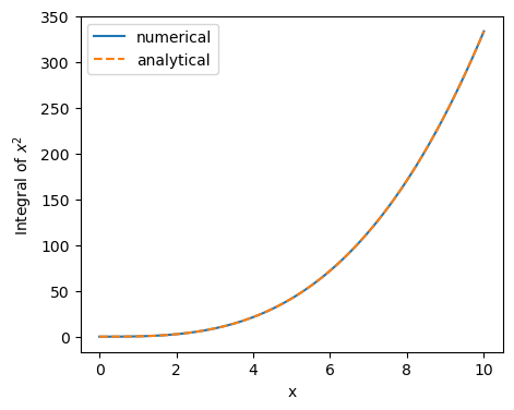
If everything went right, you should see that the two curves agree. Now that we have created some small working code, it would be worth considering to commit this with git. For explanatory purposes we’ll first do this ‘the wrong way’:

Save your file. If you use VSCode: then you can commit the file by selecting “source control” on the side-bar (or pressing “ctrl+shift+g” – on my system). Then press the plus next to the notebook file, press the commit button and write a commit message, e.g. ‘added a generic integration function to potentials.ipynb’, save (ctrl+s) and close the file (ctrl+w). To synchronize with the server click “sync changes” or select “push” from the “…” drop-down menu (next to “Changes”).

Alternatively, you can also do it from the command line. Note that the steps map one-to-one:

git add notebooks/potentials.ipynb
git status # check that the notebook has been staged correctly
git commit # write a commit message, save and close
git push   # upload our changes to github

To keep things short, from now on I will only show the command-line version, but you should always be able to figure out how to do the same thing from VSCode easily.

To appreciate what happened, open your github page (under https://github.com/[your github name]/spherical-potential). You should be able to see the “notebooks” directory and also open your new notebook file. If you download your repository on another computer with git clone ... you will directly get the newest version of the repository. If you pushed some changes on one machine and want to get the latest changes on another one, that already has the repository, you can simply do git pull.

Now let us consider a few things that are not quite optimal with what we just did:

• Our notebook file includes an image-file in its source code. This is not good:
  • This makes our notebook a relatively large file. If we commit files like this many times, then we can quickly bloat the repository. (Note that the size of the repository corresponds the cumulative size of all files that were ever committed.) This may make it difficult to work with the repository and in the worst case it may bring us to a point where we exceed the maximum online storage (e.g. ~ 500MB for a free github account.)
  • It makes it difficult to understand the history of a file, e.g. if you compare local changes via git diff
• We have written a neat little function that could in principle be used in many places. It would be much better to put it into a “.py” file and import it where we use it. This could also simplify our notebook.
• We have written a small numerical test. This is a great starting point, but it would be a great idea to formalize this test and put it into a dedicated unittest so that we can easily redo the test at any point in the future. We will discuss this in more detail in the next tutorial.

Let’s improve these things one-by-one

Stripping out notebook outputs for version control

To avoid committing the image in our notebook into our code-repository, we could simply “Clear All Outputs” every time before we commit it. It is a good idea to confirm that the whole notebook is in a reproducible state before we commit it. For this you may “Restart” and “Run All”. If everything works, “Clear All Outputs” and commit.

However, this workflow is still somewhat annoying: For example if you check with “git status” which files have changed, you will often find your notebook there, even though you did not touch any code. Further, there may be times where rerunning the notebook takes a while and you don’t want to delete all your outputs every time that you commit. A good solution to these problems is to use nbstripout. We can set this python module up as a git clean/smudge filter that will strip outputs from our notebooks before they are staged (git add) or before version differences are compared (git diff). This happens only inside git and doesn’t remove the outputs from the file that we are working with.

pip install nbstripout
# in your code-repository:
nbstripout --install --attributes .gitattributes

Here we only activated nbstripout locally for this repository. It is also possible to set it up globally if you want to use it always for all your repositories. -> see nbstripout.

Now let’s commit our changed .gitattributes and our notebook again

git add .gitattributes notebooks/potentials.ipynb
git commit -m "added usage of nbstripout"
git push

Now if you check the notebook on your github, you can see that the output has indeed been stripped, even if you committed while the outputs were still in your file.

In some cases, you may actually want to synchronize the outputs – for example if you publish your repository and you want users to be able to see the outputs online. You can easily deactivate nbstripout again: nbstripout --uninstall --attributes .gitattributes. I recommend to keep it active by default and to deactivate it temporarily for the special cases.

Extracting python functions to a module

We now have a great setup for working with notebooks. It is a good idea to commit your work frequently so that it is easy to follow what has changed. However, notebook files tend to get very large and messy quickly. Therefore, it is a good idea to extract parts into modules whenever possible.

Let us directly follow the standard python “src” layout for this. First let’s create the directory structure with pyproject.toml, src/spherical_potential/__init__.py and a python file that shall contain our actual code src/spherical_potential/integrals.py

tree --noreport -I '.git'
.
├── LICENSE
├── README.md
├── notebooks
│   └── potentials.ipynb
├── pyproject.toml
└── src
    └── spherical_potential
        ├── __init__.py
        └── integrals.py

And insert the following code into these files

import numpy as np

def cumulative_integral(fi, xi, method="trapezoidal", initial=0):
    assert method in ("trapezoidal", ), "Only 'trapezoidal' method is implemented."
    yparent = np.cumsum(0.5 * (fi[:-1] + fi[1:]) * (xi[1:] - xi[:-1]))
    return np.insert(yparent + initial, 0, initial) # add initial value

from . import integrals

[build-system]
requires = ["setuptools>=68", "wheel"]
build-backend = "setuptools.build_meta"

[project]
name = "spherical-potential"
version = "0.1.0"
description = "A library for calculating the potential of spherical mass distributions"
readme = "README.md"
requires-python = ">=3.9"
license = { file = "LICENSE" }
authors = [{ name = "[Your Name]" }]  # Fill in your name!
dependencies = ["numpy"]

[tool.setuptools.packages.find]
where = ["src"]

A bunch of things have happened here, so let’s break it down one-by-one:

• The directory “src/spherical_potential” shall be a directory that we can import as a module and “src/spherical_potential/integrals.py” shall be importable as a submodule. To define an importable directory all one has to do is to create an __init__.py inside of it. We can write code into this file to define what should happen if someone just imports the directory (import spherical_potential). We want the submodule to be imported in that case – thus the content of __init__.py
• pyproject.toml: This file declares that we are creating an installable python package. Here we can define some meta-information about our package. Most of this is not very important up to the point where you might want to publish your package on PyPI so that it is possible to install it without downloading your repository, (e.g. pip install spherical-potential). For now, the most relevant aspects are that we define that our code lies in the src directory and that numpy will be installed as a necessary dependency.

In older pip versions it was necessary to define a setup.py rather than a pyproject.toml. If you want the backwards compatibility you might need to have both files. However, I think that by now it is reasonable to require users to upgrade their outdated pip installation instead.

Now let’s install our package

pip install -e .

The “-e” installs the repository in editable mode so that modifications are immediately usable without installing the package again. You almost always want to use this option when you are developing a package.

We can now update our notebook to work with our new library:

import numpy as np
import matplotlib.pyplot as plt
import spherical_potential as sp

x = np.linspace(0, 10, 100)

plt.plot(x, sp.integrals.cumulative_integral(x**2, x), label="numerical")
plt.plot(x, x**3/3., ls='dashed', label="analytical")
plt.xlabel('x')
plt.ylabel('Integral of $x^2$')
plt.legend()

This may seem like a lot of effort for achieving the same result as earlier. However, consider that you only need to go through this setup once. When your project grows, you will benefit a lot from having a clean structure. Further, you will be able to share your library much more easily with colleagues.

Auto-reloading modules

One thing that you may immediately notice as a drawback when working with the separate module is that a change to your “.py” file does not immediately propagate to the running notebook. For example try adding a little print statement to our function

def cumulative_integral(fi, xi, method="trapezoidal", initial=0):
    print(f"Integrating with {method} method")
    assert method in ("trapezoidal", ), "Only 'trapezoidal' method is implemented."
    yparent = np.cumsum(0.5 * (fi[:-1] + fi[1:]) * (xi[1:] - xi[:-1]))
    return np.insert(yparent + initial, 0, initial) # add initial value

If you do this while your notebook is running, it will not change until you restart your notebook. This may be quite annoying when your execution takes a long time. Here to help is the %autoreload inline magic for jupyter notebooks. Simply update the first cell towards

import numpy as np
import matplotlib.pyplot as plt
import spherical_potential as sp
%load_ext autoreload
%autoreload 2

and you’ll notice that any changes to your module get immediately reloaded, whenever you save them. (This assumes that you installed with “-e”).

Let’s not forget to commit our new changes

git add src pyproject.toml notebooks/potentials.ipynb
git commit -m "Set up project as an installable python package"
git push

As a matter of good style, we should also update our README.md with some installation instructions, e.g.

# spherical-potential
This code is currently under construction. It will help with evaluating the gravitational potential of spherically symmetric mass distributions.

# Installation
To install simply do
```bash
pip install -e .
```
(You may skip the "-e" if you don't plan to edit the code)

and of course, commit the changes!

Summary

You now know how to set up a basic python/git project. I recommend that you always set up your project in this way.

You can find the final state of the repository at the end of this tutorial here

In the next tutorial we will learn how to use unit tests to verify our code. We will continue with the repository that we have set up here, but our code will grow quite a bit in complexity and it will become more obvious why we need such a structure as here.

You can also find a brief overview of useful commands and setup in this cheat sheet.