Optimizing jax.jit

Here I will discuss some low-level insights on getting the most out of jax.jit. I do not recommend going through this unless you have already a fairly good understanding of jax and jax’s just-in-time compilation jax.jit.

I highly recommend to download the code and experiment yourself.

Concepts:

• GPU kernel: A GPU program that is executed in parallel. Kernels cannot communicate directly
• Device Arrays: An array that lives in GPU RAM – usually this is the data that needs to be input, output or transferred between GPU kernels (but not the kernel-internal data.)
• Graph: An arrangement of several GPU kernels (+ their internal operations). The most important aspects are the boundaries between kernels
• temporaries: Device arrays that need to be temporarily created and passed between kernels, but that may be discarded later
• Fusing: Grouping of several operations as internal operations inside of a kernel / Merging of kernels to reduce the number of kernel launches
• Fusion Barriers: Some operations prevent that code before and after them can be fused into one kernel, e.g. FFTs, reduction operations (jnp.sum), …

Introduction: Understanding Graphs

x = jnp.zeros((1024*128,2)) # uses 1MB

def kvec_mesh(N):
    return jnp.stack((jnp.arange(0, N), jnp.arange(0, N)), axis=-1)

def f_sum_jax(x):
    kvm = kvec_mesh(len(x))
    return x * 2 + jnp.sum(kvm * x, axis=1, keepdims=True)

show_hlo_info(jax.jit(f_sum_jax), x, width=500)

--------  Memory usage of f_sum_jax  ---------
code  : 5.1 kB
temp  : 512.0 kB
arg   : 1.0 MB
output: 1.0 MB
alias : 0 B
peak  : 2.5 MB

Graph Details This is a wild guess, the colors in the graph might roghly represent the following:

• Orange boxes: input parameters of the full graph or of kernels
• White boxes: operations that preserve shapes
• Green boxes: operations that have a larger output size than input size
• Purple boxes: reduction operations that have smaller output than input size
• Yellow boxes: operations that modify the shape, but not the size
• Blue boxes: external library calls
• Large grey boxes: kernels
• Large white boxes: “Subcomputations” that may group several kernels together.
• Arrows between kernels: Arrays that are passed through device memory (GPU RAM)
• Arrows inside kernels: Variables of the kernel that live in registers (i.e. an array that does not need to be materialized in GPU RAM)

Above you can see an example of a Graph. The grey boxes indicate the boundaries of different kernels. Inside of each kernel you can see all the operations that jax managed to “fuse” together. There is a lot of information in the graph… what should we focus on?

Most GPU programs tend to be limited by memory-bandwidth. Therefore the main performance consideration is not the complexity of the internal computation, but rather the amount of data that needs to be input and output.

As a good baseline, assume that all internal computations inside a kernel are for free. Performance cost is dominated by the size of the inputs and outputs of each kernel. Memory size is dominated by the number of temporary arrays that may need to be kept at once.

The only relevant aspects of the graph are then:

• How many kernels are used (because of memory bandwidth and kernel launch overhead)
• How many arrows (of which size) appear between the kernels

Our goal when optimizing jax.jit is then generally to write our instructions in such a way that it allows jax.jit to minimize the number of kernels and to minimize the amount of data transferred between them – or to maximize fusion. This can in practice be achieved by avoiding fusion barriers and by preferring to recalculate intermediate results instead of saving them in temporaries.

For example in the graph above, two kernels are required. Between the two kernels a temporary array with half the size of x is passed through device memory. (Therefore, the temporary allocation of 512KB.) This graph is sub-optimal (as we shall show later), because it would have been possible to fuse everything into a single kernel with zero temporaries. This requires that we write our code in a way that respects XLA’s limitations. Unfortunately these are not really documented at all and we can only learn them by conducting experiments.

Below we will go through a notable number of experiments to understand what type of computation can or cannot be fused. If you are only interested in the key-takeaways, consider jumping directly to the summary.

Fusing

In general jax does a really good job at fusing (and not creating temporaries). Especially operations where each output element can be calculated from a single input element always get fused optimally in jax.

x = jnp.zeros((1024*128,2)) # uses 1MB

def f_well_fused(x):
    a = x * 2
    b = jnp.arange(a.shape[0])[:,None] * 3
    c = x[0] + x - a
    return jnp.sin(a) + a**2 + b + c

show_hlo_info(jax.jit(f_well_fused), x, width=500)

--------  Memory usage of f_well_fused  ---------
code  : 11.4 kB
temp  : 0 B
arg   : 1.0 MB
output: 1.0 MB
alias : 0 B
peak  : 2.0 MB

Fusion barriers

Some operations cannot fuse, effectively creating “barriers”. There is no 100% way of identifying them without testing it. However, a good guideline is that if an operation requires a library call or if the operation’s input and output layout mismatch, then it may prevent fusion. For example, below we use jnp.sum(…, axis=1) to calculate the dot product between two arrays and this stops the fusion. In the scenario here, we can avoid jnp.sum by explicit summation and we recover a single fused kernel, saving temporary memory and performance.

def kvec_mesh(N):
    return jnp.stack((jnp.arange(0, N), jnp.arange(0, N)), axis=-1)

def f_sum_jax(x):
    kvm = kvec_mesh(len(x))
    return x * 2 + jnp.sum(kvm * x, axis=1, keepdims=True)

def f_sum_explicit(x):
    kvm = kvec_mesh(len(x))
    return x * 2 + (kvm[...,0] * x[...,0] + kvm[...,1] * x[...,1])[:,None]

x = jnp.zeros((1024*128,2)) # uses 1MB
show_hlo_info(jax.jit(f_sum_jax), x)
show_hlo_info(jax.jit(f_sum_explicit), x)

--------  Memory usage of f_sum_jax  ---------
code  : 5.1 kB
temp  : 512.0 kB
arg   : 1.0 MB
output: 1.0 MB
alias : 0 B
peak  : 2.5 MB

--------  Memory usage of f_sum_explicit  ---------
code  : 3.4 kB
temp  : 0 B
arg   : 1.0 MB
output: 1.0 MB
alias : 0 B
peak  : 2.0 MB

jitting sub functions

Differently than I would have expected, sub-functions do not prevent fusion!

def finternal(x):
    return x * 2 + 25.0
finternal.jit = jax.jit(finternal, inline=False)

def f_with_subjit(x):
    return finternal.jit(x) + 3

show_hlo_info(jax.jit(f_with_subjit), x, width=300)

Note, how even the 25 was fused with the 3 into a single addition of 28!

Intentional Fusion barriers

It is possible to explicitly prevent fusion and common subexpression elimination (later more about this) by inserting jax.lax.optimization_barrier. This is what jax’s rematerialization may try to do to reduce memory usage in extreme scenarios.

def f_with_subjit(x):
    """Becomes two kernels, because we have a barrier in between"""
    S = jax.lax.optimization_barrier(jnp.sin(x) + 3)
    return S + jnp.exp(S)

show_hlo_info(jax.jit(f_with_subjit), x, width=300) 

--------  Memory usage of f_with_subjit  ---------
code  : 13.1 kB
temp  : 0 B
arg   : 1.0 MB
output: 1.0 MB
alias : 0 B
peak  : 2.0 MB

Note that jax does a pretty good job in avoiding temporary arrays here. I.e. even although it needs to pass 1MB of data between the kernels, it does not require any additional temporary allocation. I think that jax likely uses the final output array as an intermediate storage and then lets the second kernel operate in place. Operations that cannot work in-place (e.g. transpositions) may need a temporary array in situations like this.

FFTs

Fast Fourier transformations are probably implemented in XLA through library calls and always create a fusion barrier. It seems the library that jax calls assumes that batched FFTs shall be batched across the first dimension. (This also makes sense, from a CUDA perspective.) Therefore, if you start with an (N,N,N,2) layout the graph becomes more complicated than if you start with (2,N,N,N):

def f_fft3d(x):
    a = jnp.fft.rfftn(x, axes=(0,1,2))
    b = jnp.fft.irfftn(a, axes=(0,1,2))
    return b

def f_fft3d_transposed(x):
    a = jnp.fft.rfftn(x, axes=(1,2,3))
    b = jnp.fft.irfftn(a*2, axes=(1,2,3))
    return b + 3

x3d = jnp.zeros((64,64,32,2)) # Our probe array -- it uses 1MB
show_hlo_info(jax.jit(f_fft3d), x3d, width=250)
show_hlo_info(jax.jit(f_fft3d_transposed), x3d.transpose(3,0,1,2), width=250)

--------  Memory usage of f_fft3d  ---------
code  : 5.1 kB
temp  : 2.1 MB
arg   : 1.0 MB
output: 1.0 MB
alias : 0 B
peak  : 4.1 MB
--------  Memory usage of f_fft3d_transposed  ---------
code  : 5.2 kB
temp  : 1.1 MB
arg   : 1.0 MB
output: 1.0 MB
alias : 0 B
peak  : 3.1 MB

The memory usage of the second version is smaller, because no transpose is needed. To transpose a temporary array (which has to be done in Fourier space), two temporaries are needed, one for the input and one for the output. Therefore the first kernel needs ~2MB, but the second only 1MB. Note that this doesn’t get affected by any in-place modifications which generally do not create temporaries (as discussed above).

Loops

Loops in jax are implemented as multiple successive kernel launches. (Note that the loop is not fused into the kernel – as would be possible in CUDA. I wonder whether it is somehow possible to achieve such a fusion, e.g. in the case below.) Each iteration launches a kernel. It is possible to fuse neighboring loop iterations by unrolling them – partially or fully. If you fully unroll a loop, you may even achieve a single fused kernel. (Probably this is equivalent to a python compile-time loop.)

def f_for(x, unroll=None):
    def add_x(i, x):
        return x*x + 1
    y = jax.lax.fori_loop(0, 4, add_x, x, unroll=unroll)
    return y

show_hlo_info(jax.jit(f_for, static_argnames="unroll"), x, width=800)
# Partially unrolled, saves half of the kernel launches and I/O, but still needs a temporary
show_hlo_info(jax.jit(f_for, static_argnames="unroll"), x, unroll=2, width=800)
# Fully unrolled, becomes a single kernel avoids 1 temporary:
show_hlo_info(jax.jit(f_for, static_argnames="unroll"), x, unroll=4, width=200)

--------  Memory usage of f_for  ---------
code  : 6.9 kB
temp  : 513 B
arg   : 1.0 MB
output: 1.0 MB
alias : 0 B
peak  : 2.0 MB

--------  Memory usage of f_for  ---------
code  : 7.2 kB
temp  : 513 B
arg   : 1.0 MB
output: 1.0 MB
alias : 0 B
peak  : 2.0 MB

--------  Memory usage of f_for  ---------
code  : 3.7 kB
temp  : 0 B
arg   : 1.0 MB
output: 1.0 MB
alias : 0 B
peak  : 2.0 MB

Common sub-expression elimination (CSE)

The handling of common sub-expressions is probably the most difficult to comprehend part of jax’s optimization strategies. At the same time it may be one of the most relevant aspects, since it can greatly affect memory usage and I/O performance.

Consider the following two almost identical functions:

def f_recalc(x):
    im = jnp.exp(jnp.arange(x.size).reshape(x.shape) ** 2.3)

    # Here we use a sum to create a fusion barrier
    # Imagine this represents a long calculation that cannot be fused
    a = x + jnp.sum(im, axis=-1, keepdims=True) 

    # Later we use "im" again. Does jax store the result to reuse it here or recalculate it?
    return a + im 

def f_stored(x):
    im = jnp.sin(jnp.arange(x.size).reshape(x.shape) ** 2.3) # only difference jnp.exp -> jnp.sin
    a = x + jnp.sum(im, axis=-1, keepdims=True) 

    return a + im

show_hlo_info(jax.jit(f_recalc), x, width=700)
show_hlo_info(jax.jit(f_stored), x, width=700)

There is only a tiny difference (jnp.sin instead of a jnp.exp) in the second function. However, the graphs turn out very different:

Note that the second graph calculates the intermediate expression once and the passes it (together with the result of jnp.sum) to the next kernel. The first graph instead reevaluates the expression in the second kernel. As discussed in the beginning, this is in most scenarios the behaviour that we prefer.

I have no clue why this difference in the graph was triggered by a simple switch from jnp.sin to jnp.exp. However, it is clear that jax uses some heuristics that we cannot predict. If we had a more complicated scenario, the second case might require significantly more memory. I find such an arbitrary behaviour very bad for writing good high performance computing (HPC) code. That’s why I created a feature request on jax’s GitHub for a clear way to control this. Let’s see whether they take this seriously.

As of now I couldn’t find a clean way to have kernel 2 behave identically to kernel 1. There is a hacky way though, by recomputing im on the second use with an epsilon difference.

PS: There exists an experimental XLA flag --xla_gpu_experimental_collective_cse_distance_threshold. I tried it, but it didn’t seem to have any effect in the scenario at hand…

Anyways… the problem may come up less than we might expect. Most calculations seem to be sufficiently cheap that jax will redo them automatically. Also the “scoping aspect”, that we will discuss next, can help us avoid much of the problem.

CSE and scoping

It appears that repeating the same sub-expression is not always identical to defining a tracer with the sub-expression once and reusing it. Consider the following examples:

def get_im(x, eps=0.):
    return jnp.sin((jnp.arange(x.size).reshape(x.shape) + eps) ** 2.3)

def f_cse(x):
    a = x + jnp.sum(get_im(x), axis=-1, keepdims=True) 

    b =  jnp.sum(a + get_im(x))

    return a + get_im(x) + b

Here jax finds a common sub-expression and calculates it once:

def f_cse_loop_expl(x):
    im = get_im(x)

    def step(i, a):
        return a + im

    return jax.lax.fori_loop(0, 5, step, x + im)

Here it does, too (and passes it as a second input into the loop):

However, here we recreate the sub-expression inside of the loop:

def f_cse_loop_impl(x):
    """Here it does not find the common sub-expression, it will be recalculated
    Likely loops live in a different scope and CSE does not identify sub-expressions across scopes
    (this is actually what we want! Uses less memory)"""
    def step(i, a):
        return a + get_im(x)

    return jax.lax.fori_loop(0, 5, step, x + get_im(x))

and jax does not find a common sub-expression and therefore it recalculates our temporary in every iteration.

(Remember: this is the behaviour we prefer!) We can see the advantage in the memory report – our third variant basically using no temporary memory:

--------  Memory usage of f_cse  ---------
code  : 37.8 kB
temp  : 514.3 kB
arg   : 1.0 MB
output: 1.0 MB
alias : 0 B
peak  : 2.5 MB

--------  Memory usage of f_cse_loop_expl  ---------
code  : 20.5 kB
temp  : 1.0 MB
arg   : 1.0 MB
output: 1.0 MB
alias : 0 B
peak  : 3.0 MB

--------  Memory usage of f_cse_loop_impl  ---------
code  : 31.8 kB
temp  : 513 B
arg   : 1.0 MB
output: 1.0 MB
alias : 0 B
peak  : 2.0 MB

Note that before and after the loop lie in the same “scope” again:

def f_cse_loop_after(x):
    """Finds a common sub-expression between pre-and post-loop... increase memory again..."""
    def step(i, a):
        return a + get_im(x)

    return jax.lax.fori_loop(0, 5, step, x + get_im(x)) + get_im(x) # if we pass eps = 1e-10 here, it will not find it though

Here the expression is reevaluated inside the loop, but a temporary is created to connect its usage before and after the loop:

--------  Memory usage of f_cse_loop_after  ---------
code  : 40.5 kB
temp  : 1.0 MB
arg   : 1.0 MB
output: 1.0 MB
alias : 0 B
peak  : 3.0 MB

From these examples I suggest the following guidelines:

Since recalculation is almost always better than having a temporary array (especially if it can be fused into the kernel), the following approach will likely be as-good-as-it-gets in most cases:

• For every “array” that can be cheaply recalculated define a (pure jax) function
• Wherever you need it, call the function
• In 90% of cases this should lead to consistent recalculation and be optimal
• For the other 10% it may be worth it to inspect the graph and see whether it actually gets recalculated in each kernel
• If XLA decides to create a temporary, (happens if the calculation is sufficiently expensive and two calls to the function exist in the same scope, but cannot be fused) for now, the only way out is to make it unidentifiable as a common sub-expression: E.g. each time you reuse the variable modify its calculation by a different epsilon.

How to optimally evaluate a Fourier k-mesh

A good example of a common sub-expression that we always want to reevaluate is the $k$-vector grid in Fourier space. In most cases we need only the absolute value of the $k$-vector. Below I show you two implementations of it, one being clearly better (after inspection).

The naive implementation

def get_kmesh_naive(rho, d=1., norm2=True, real=True):
    """In general d=boxsize/(2*np.pi*rho.shape[0])"""
    kx = jnp.fft.fftfreq(rho.shape[0], d=d)
    ky = jnp.fft.fftfreq(rho.shape[1], d=d)
    if real:
        kz = jnp.fft.rfftfreq(rho.shape[2], d=d)
    else:
        kz = jnp.fft.fftfreq(rho.shape[2], d=d)

    kx,ky,kz = jnp.meshgrid(kx, ky, kz, indexing="ij")
    if norm2:
        return kx**2 + ky**2 + kz**2
    else:
        return jnp.stack((kx,ky,kz), axis=-1)

leads for norm2=True to the following graph with two kernels… I can only guess why this happens. Possibly the dispatch layout of jnp.meshgrid is different than the one that is preferred for the subsequent $k^2$ calculation.

However, if we write the function in a way that enforces the layout in which we want our outputs, we get a single kernel:

def myfftfreq(i, n, d=1.0):
    """Does the same as jnp.fft.fftfreq(n, d)[i] but avoids creating the frequency array"""
    return jnp.where(i < (n+1)//2, i / n, (i - n)/n) / d
def myrfftfreq(i, n, d=1.0):
    """Does the same as jnp.fft.rfftfreq(n, d)[i] but avoids creating the frequency array"""
    return i / n / d

def get_kmesh(rho, d=1., norm2=False, real=True):
    ix,iy,iz = jnp.indices((rho.shape[0], rho.shape[1], (rho.shape[2]//2)+1 if real else rho.shape[2]))
    
    kx = myfftfreq(ix, rho.shape[0], d=d)
    ky = myfftfreq(iy, rho.shape[1], d=d)
    
    if real:
        kz = myrfftfreq(iz, rho.shape[2], d=d)
    else:
        kz = myfftfreq(iz, rho.shape[2], d=d)

    if norm2:
        return kx**2 + ky**2 + kz**2
    else:
        return jnp.stack((kx,ky,kz), axis=-1)

Again: this is much better!

With this implementation we can do the filtering in Fourier space with a single dispatch and no temporary arrays! For example:

def f_filter_with_recalc(rho):
    def step(i, rho):
        rhok = jnp.fft.rfftn(rho, axes=(0,1,2))
        rhok *= jnp.exp(-0.5 * get_kmesh(rho, norm2=True))
        return jnp.fft.irfftn(rhok, axes=(0,1,2))

    return jax.lax.fori_loop(0, 5, step, rho)

--------  Memory usage of f_filter_with_recalc  ---------
code  : 9.2 kB
temp  : 1.0 MB
arg   : 1.0 MB
output: 1.0 MB
alias : 0 B
peak  : 3.0 MB

Our operation gets fused into the same code that multiplies the filter with rhok this is exactly what we want. A CUDA kernel wouldn’t be more optimal than this!

Constant folding

The worst of all evils in jax is constant folding. You should avoid it at all costs. Folded constants appear as ‘code_size’ in the memory report. They live in device memory space and they contribute to peak memory! Also they absolutely obliterate compilation time:

E.g. compare the two functions:

import numpy as np
def f_numpy(x):
    return x + np.arange(x.size).reshape(x.shape) ** 2.3 # np array gets always folded

def f(x):
    return x + jnp.arange(x.size).reshape(x.shape) ** 2.3

x2 = jnp.zeros((1024*1024*16,2)) # Our probe array -- it uses 128MB
show_hlo_info(jax.jit(f_numpy), x2)  # takes >5s to compile, scaling with the size of the constant
show_hlo_info(jax.jit(f), x2)

--------  Memory usage of f_numpy  ---------
Warning! We have constant folding!
code  : 128.0 MB
temp  : 0 B
arg   : 128.0 MB
output: 128.0 MB
alias : 0 B
peak  : 384.0 MB

--------  Memory usage of f  ---------
code  : 7.5 kB
temp  : 0 B
arg   : 128.0 MB
output: 128.0 MB
alias : 0 B
peak  : 256.0 MB

In the graph, folded constants appear very subtle:

Parallel execution

Jax tries to schedule calculations in parallel if it can. Consider the following function:

def f_fft_multi(x, n=5):
    res = 0
    for i in range(n):
        res = res + jnp.fft.irfftn((i+2)*jnp.fft.rfftn(x+i, axes=(1,2,3)), axes=(1,2,3))**(i+2)
    return res
f_fft_multi.jit = jax.jit(f_fft_multi, static_argnames="n")

With n=3:

The three FFTs can all be calculated in parallel and later added together. In theory, if each calculation uses only a small fraction of the GPU (e.g. very small array sizes <~ 1MB), then this could have a big benefit, since we can fill any idlle processors for free. When each calculation is large (e.g. array sizes 100s of MB) then the performance benefit might be less relevant. So much the theory… In practice, I haven’t been able to measure any benefits of this. (See experiments below.)

On the other hand, parallel scheduling will strongly increase memory usage. It is therefore useful to know how to prevent it, if we encounter a situation where memory usage is important.

We can force sequential execution…

• …with a for loop (works only here, where we have a loop)
• …with optimization_barriers (can be used in any scenario!)

Quoting the jax documentation: “An optimization barrier ensures that every output of the barrier that is used by any operator, has been evaluated before any operator that depends on one of the barrier’s outputs. This can be used to enforce a particular order of operations.”

So we can ensure sequential execution by making the inputs of the other operators depend on something in the optimization barrier – e.g. x!

def f_fft_multi_for(x, n=5):
    def step(i, res):
        return res + jnp.fft.irfftn((i+2)*jnp.fft.rfftn(x+i+1, axes=(1,2,3)), axes=(1,2,3))**(i+2)
    return jax.lax.fori_loop(0, n, step, jnp.zeros_like(x))
f_fft_multi_for.jit = jax.jit(f_fft_multi_for, static_argnames="n")

def f_fft_multi_barrier(x, n=5):
    res = 0
    for i in range(n):
        res = res + jnp.fft.irfftn((i+2)*jnp.fft.rfftn(x+i, axes=(1,2,3)), axes=(1,2,3))**(i+2)
        res,x = jax.lax.optimization_barrier((res, x))
    return res
f_fft_multi_barrier.jit = jax.jit(f_fft_multi_barrier, static_argnames="n")

x3d = jnp.zeros((2,64,64,32)) # Put 2000 here if you want to see "rematerialization" fail
ns = np.arange(1, 10, dtype=int)
nbytes = np.array([f_fft_multi.jit.lower(x3d, n=n).compile().memory_analysis().temp_size_in_bytes for n in ns])
nbytes_for = np.array([f_fft_multi_for.jit.lower(x3d, n=n).compile().memory_analysis().temp_size_in_bytes for n in ns])
nbytes_opt = np.array([f_fft_multi_barrier.jit.lower(x3d, n=n).compile().memory_analysis().temp_size_in_bytes for n in ns])

plt.xlabel("n (number of parallel executable FFTs)")
plt.ylabel("Temporary memory usage [MB]")
plt.plot(ns, nbytes/1e6, marker="o", label="python loop")
plt.plot(ns, nbytes_for/1e6, marker="o", label="jax for loop")
plt.plot(ns, nbytes_opt/1e6, marker="x", label="barriers", ls="dashed")
plt.legend()

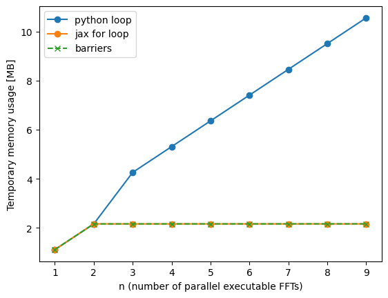
Note how we drastically reduced the memory usage with the help of the barrier (or the loop). Obviously we can also use the trick with the barrier in more complex scenarios with multiple branches that are not identical.

Note: in principle, jax’s “rematerialization” is intended to solve memory problems and rearrange computations with barriers, just as we did here. In practice I have never found it to work properly though… E.g. in the example below we can get away with 2x temporaries, but rematerialization never achieves this… For now we should never rely on rematerialization to fix our memory problems.

Now let’s see whether we lose any performance here:

# Extremely small array
x3d = jnp.zeros((2,16,16,16)).block_until_ready()
%timeit -n 100 f_fft_multi.jit(x3d, n=5).block_until_ready()
%timeit -n 100 f_fft_multi_for.jit(x3d, n=5).block_until_ready()
%timeit -n 100 f_fft_multi_barrier.jit(x3d, n=5).block_until_ready()

# Intermediate array
x3d = jnp.zeros((20,64,64,32))
%timeit -n 100 f_fft_multi.jit(x3d, n=5).block_until_ready()
%timeit -n 100 f_fft_multi_for.jit(x3d, n=5).block_until_ready()
%timeit -n 100 f_fft_multi_barrier.jit(x3d, n=5).block_until_ready()

# Large array
x3d = jnp.zeros((200,64,64,32))
%timeit -n 100 f_fft_multi.jit(x3d, n=5).block_until_ready()
%timeit -n 100 f_fft_multi_for.jit(x3d, n=5).block_until_ready()
%timeit -n 100 f_fft_multi_barrier.jit(x3d, n=5).block_until_ready()

1.59 ms ± 50.8 μs per loop (mean ± std. dev. of 7 runs, 100 loops each)
1.77 ms ± 80.9 μs per loop (mean ± std. dev. of 7 runs, 100 loops each)
1.71 ms ± 37.6 μs per loop (mean ± std. dev. of 7 runs, 100 loops each)

2.9 ms ± 16.2 μs per loop (mean ± std. dev. of 7 runs, 100 loops each)
2.81 ms ± 39.5 μs per loop (mean ± std. dev. of 7 runs, 100 loops each)
2.68 ms ± 28.2 μs per loop (mean ± std. dev. of 7 runs, 100 loops each)

51.1 ms ± 1.14 ms per loop (mean ± std. dev. of 7 runs, 100 loops each)
57.8 ms ± 390 μs per loop (mean ± std. dev. of 7 runs, 100 loops each)
55.3 ms ± 603 μs per loop (mean ± std. dev. of 7 runs, 100 loops each)

The measurements don’t give a terribly clear picture. The strategy with barriers seems to perform at worst 10% worse and at best even 10% better than the parallel-scheduled one. Considering the large memory benefit, I’d consider this as a good tradeoff in most cases. Of course this might be different for other computations and it is a good idea to profile your code before and after inserting barriers!

Summary

Here a quick recap of the most important things worth remembering:

• Minimize temporary memory usage
• Minimize kernel launches / Maximize fusion
• Recomputing intermediates inside of a kernel is very cheap and almost always better than keeping temporaries in device memory.
• Some operations can create fusion barriers (e.g. jnp.sum or jnp.fft.rfftn)
• Using jax.jit in a sub-function does not create a fusion barrier (I.e. it is safe, but might waste tiny amount of compilation time)
• For cheap-to-calculate “constants” that you use many times (e.g. a kmesh), prefer to put them into functions that you call for each usage. This is especially important for achieving recalculation inside of loops
• Sometimes we might need to trick jax into doing the recomputation rather than saving intermediates as temporaries
• Avoid constant folding at all costs!

Important details

Here a quick recap of some important, but surprising details that we have learned:

• Avoid reduction operators (if possible), they will generally not be fused.
• Kernels with aligned input and output work effectively in place, not needing an additional temporary array. Therefore, they never have any impact on memory usage!
• Kernels where input and output misalign – e.g. transposition kernels – cannot work in place and generally need an additional temporary array.
• Often the same holds for external library kernels (e.g. ffts or sort)
• For FFTs with vectorial data prefer (3,N,N,N) layout over (N,N,N,3) layout, since (3,N,N,N) requires no transpositions on jax’s side (internally they do, but whatever library jax calls does a better job with the memory usage)
• Jax loops can be partially unrolled to allow fusion. This may be worth it when the kernel that is looped over is very cheap (so that launch and I/O overhead dominate)
• XLA does Common Sub Expression elimination (CSE) that finds identical expressions. This is very useful in many scenarios, but it creates a nightmare for writing stable and memory-optimal code:
  • If the same expression appears more than once inside the same scope, jax identifies it and treats it as if it was the same tracer
  • If the computation is sufficiently complex, xla prefers to store it in a temporary device array from where it is first to where it is last needed (e.g. random numbers tend to be in this category)
  • If it is a reasonably simple expression, xla prefers to recalculate it locally inside of each kernel (no memory required) (e.g. jnp.arange or a kmesh Fourier Grid)
  • The boundary between the two cases is somewhat unpredictable and may be crossed because of tangible changes (e.g. in one example using jnp.sin instead of jnp.exp).
  • The CSE seems to only apply inside of the same “scope”. E.g. if you declare a tracer outside of a loop and use it in the loop, it will never be recalculated in the loop always creating a temporary (avoid this!)
  • If you redefine the computation inside of the loop and outside of the loop, it will always be recalculated inside of the loop. (So recreating a tracer, e.g. through a function, will have a different effect than reusing an identical tracer.)
  • As of now, jax does not offer a way to deactivate CSE selectively. So beyond the scoping constraints the only way to guarantee recomputation may be to try to trick jax. (Note: jax.lax.optimization_barrier does too much, it also deactivates fusion, which is generally unacceptable. jax.remat(... prevent_cse=True) seems to only apply to a gradient pass and not do anything in a normal computation). I created a feature suggestion here… let’s see what will happen
• Since recalculation is almost always better than having a temporary array (especially if it can be fused into the kernel), the following approach will likely be as-good-as-it-gets in most cases:
  • For every “constant” that can be cheaply recalculated define a (pure jax) function. E.g. get_kmesh(N) or so
  • Wherever you need the constant, call the function
  • In 90% of cases this should lead to consistent recalculation and be optimal
  • For the other 10% it may be worth it to inspect the graph and see whether it actually gets recalculated in each kernel
  • If XLA decides to create a temporary, (happens if the calculation is sufficiently expensive and two calls to the function exist in the same scope, but cannot be fused) for now, there is only one hacky way out:
  • Each time you reuse the variable modify its calculation by a different epsilon so that the expressions cannot be identified.
• Sometimes creating a meshgrid with the help of jnp.indices can be better than using jnp.meshgrid + reductions. This way we can often ensure that the kernel is launched in the right layout and avoid a fusion barrier.
• Folded constants (e.g. trace-time-known numpy arrays) contribute to device memory usage. They appear under generated_code_size_in_bytes in fcompiled.memory_analysis(). Avoid large folded constants (>1MB) at all costs!
• Parallel scheduling in graphs can very strongly affect memory usage. Rematerialization doesn’t solve it. Explicit barriers can greatly reduce memory usage at tangible performance costs (<10%).

Other Ressources

• For an overview of all available XLA flags check Lukas Winkler’s homepage.
• The article arXiv:2301.13062 investigates operator fusion in XLA and explores some optimization strategies. It inspired the experiments in this post.